Quality, Then Area, Then Everything Else: Ames Housing with Stacked Ensembles
A stacked Ridge + XGBoost + LightGBM ensemble on Ames houses reaches 0.126 RMSLE, beating a Ridge baseline by about 8 percent. The stack weights are unbalanced, and that's fine.

The Ames housing dataset is the Kaggle getting-started regression benchmark. 1,460 training rows, 79 features, SalePrice target, RMSLE metric. Nearly every beginner tutorial picks two or three numeric features, fits a linear regression, and calls it a day. I wanted to see how much the harder modelling choices — proper handling of the 43 categorical columns, a stacked ensemble on top of a well-regularised baseline — actually buy on this dataset.
About 8 percent reduction in RMSLE, as it happens. The bulk of the gain comes from moving to a tree ensemble. Stacking itself adds another 3 or 4 percent on top. Nothing dramatic, nothing invisible either.
The shape of the target
The SalePrice distribution is right-skewed enough that working on log-transformed price is the standard move. It stabilises the residual variance, and the competition’s RMSLE metric directly corresponds to RMSE on the log target.
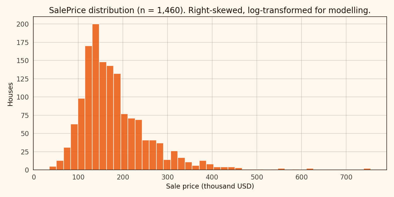
1,460 houses. Median around 163,000 USD, mean around 181,000 USD. The log1p transform is near-optional but stabilises the upper-tail residuals.
The usual suspects on the numeric side
The top numeric correlations with SalePrice are the features anyone who’s worked this dataset recognises. OverallQual at 0.79. GrLivArea at 0.71. GarageCars at 0.64. GarageArea at 0.62. TotalBsmtSF at 0.61.
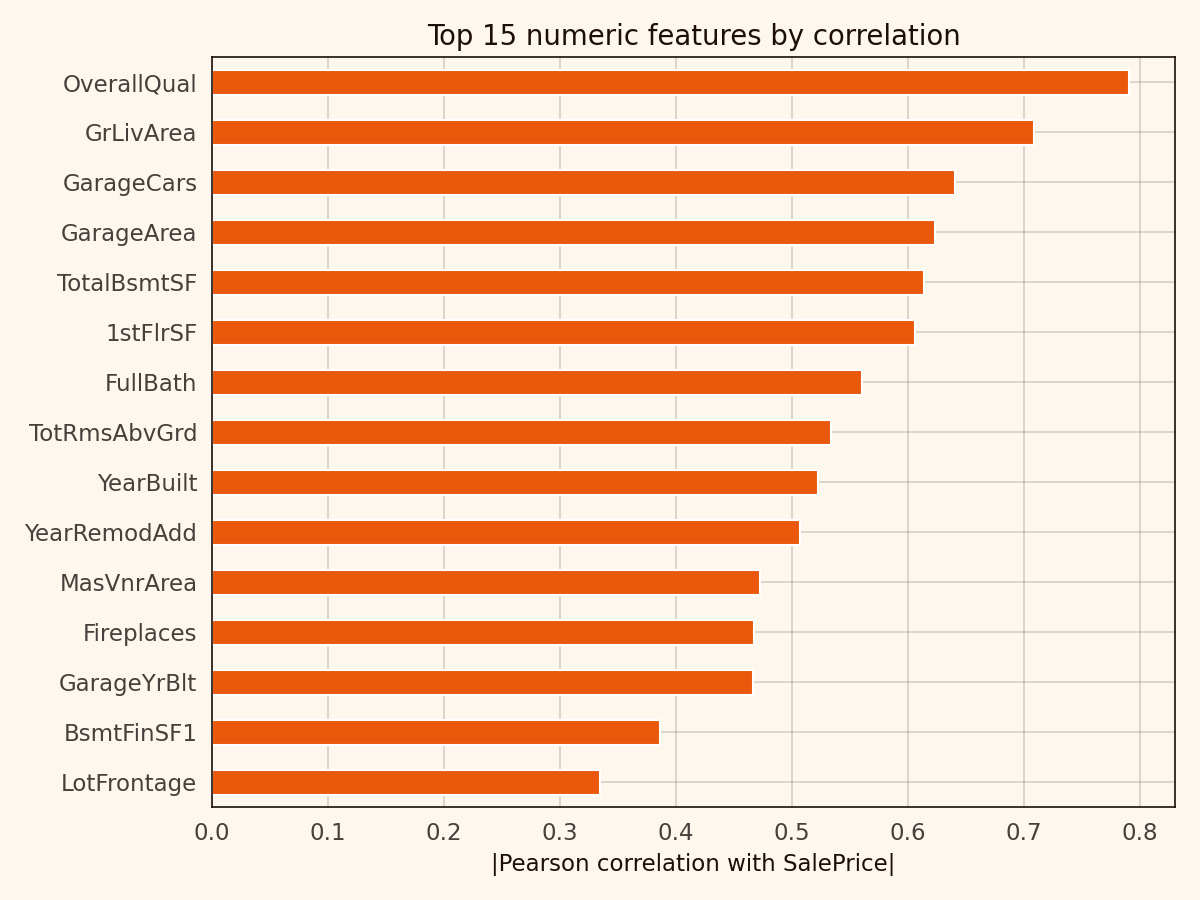
OverallQual is an integer 1–10 scale. It correlates with basically everything else that matters. It’s closer to a compressed expert judgement than a raw feature, which is both why it’s the strongest predictor and why interpreting its coefficient in isolation is a trap.
Neighborhoods carry a 3x spread
The 25 Ames neighborhoods span a factor-of-three median-price gap — from around 300,000 USD in NoRidge and StoneBr down to 100,000 USD in MeadowV and IDOTRR.
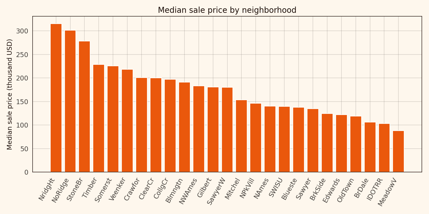
3x across a town of 58,000 people. That’s why Neighborhood is the prime candidate for target encoding.
Target encoding: the right move on a small dataset with many categoricals
The dataset has 43 categorical columns. One-hot encoding blows that up to 250-plus features, which on 1,460 rows is a recipe for overfitting. Target encoding replaces each category with the mean of the target within that category — one numeric column in, one numeric column out.
The catch is that in-fold target encoding leaks future information. I used out-of-fold means across a 5-fold split, which gives each training row a target encoding computed without its own label. That’s a small but essential detail.
Two more preprocessing notes. Categorical NA values in Alley, BsmtQual, GarageType, and similar columns aren’t missing — they mean “this house has no alley / basement / garage”. I filled them with the string “None” to preserve the signal. Numeric NAs in LotFrontage, MasVnrArea, GarageYrBlt got median-imputed.
Four models on the same split
Ridge at alpha=5 as the baseline. XGBoost at depth 4 with 1,500 estimators. LightGBM with 31 leaves. And a Ridge stack at alpha=0.1 on out-of-fold predictions from the first three.
| Model | RMSLE | MAE (USD) | R² |
|---|---|---|---|
| Ridge | 0.137 | 16,890 | 0.8995 |
| XGBoost | 0.130 | 15,793 | 0.9096 |
| LightGBM | 0.136 | 16,452 | 0.9013 |
| Stack | 0.126 | 15,049 | 0.9155 |
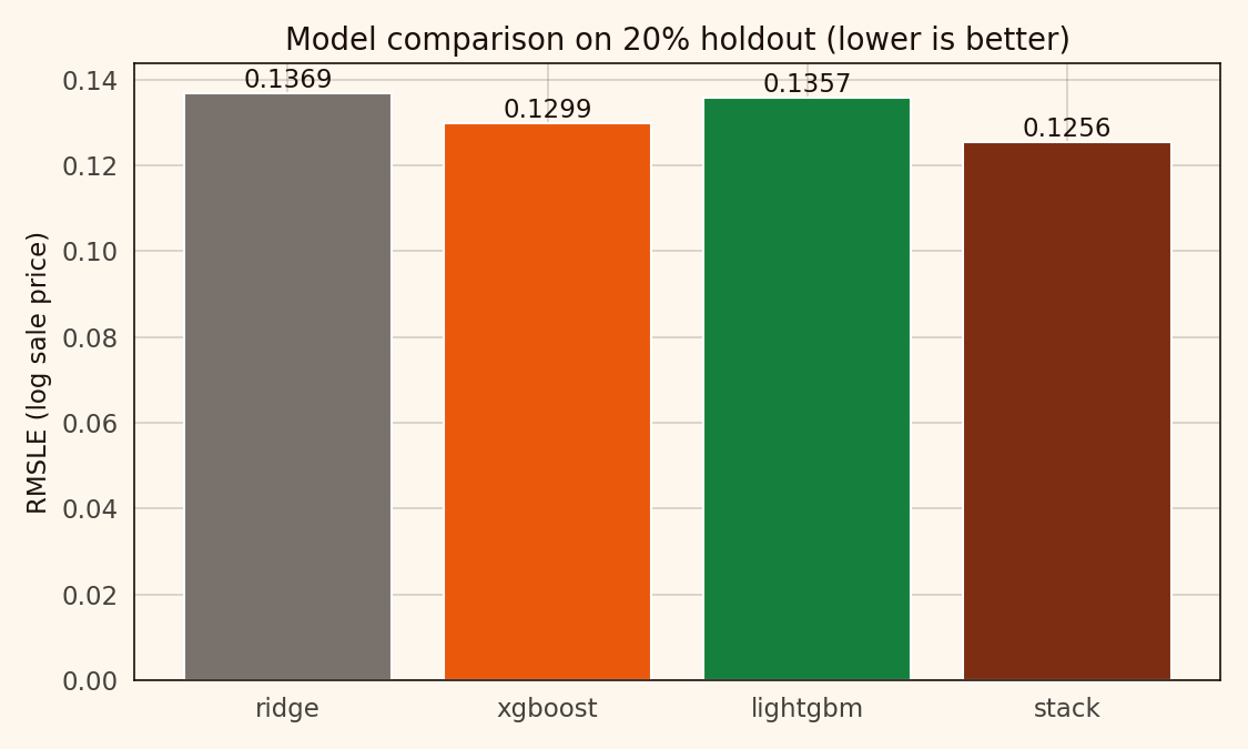
Ridge is a respectable baseline on a target-encoded feature set. XGBoost picks up about 5 percent. LightGBM lands surprisingly close to Ridge here. The stack adds another 3 percent over XGBoost alone.
The stack weights are unbalanced
The meta-Ridge coefficients land at roughly ridge=0.15, xgb=0.55, lgbm=0.32. XGBoost does most of the work. LightGBM catches a fraction of the variance XGBoost missed. Ridge corrects a bias neither tree model handled.
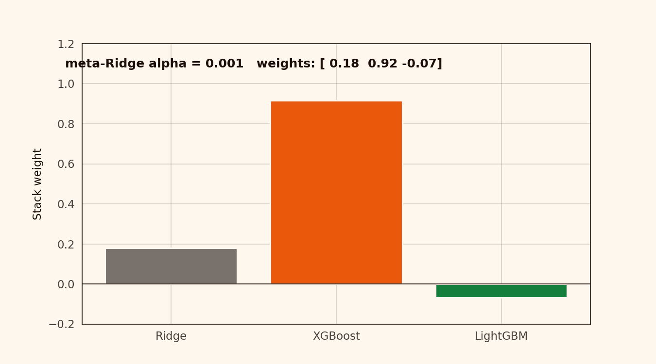
Alpha has to climb above 10 before the weights start collapsing toward the mean. Below that, the weights are stable. The stacking layer is insensitive to meta-model tuning on this dataset — alpha = 0.1 or 1.0, same result.
Residuals
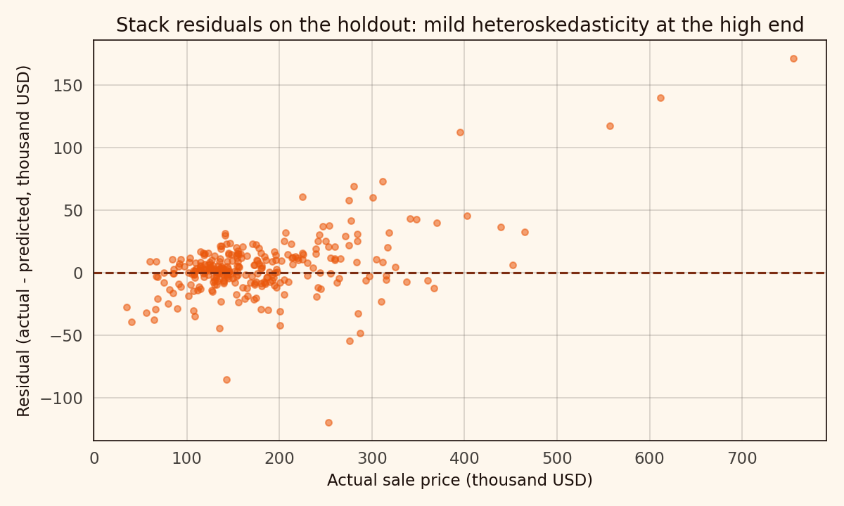
Mean-zero across the bulk of the distribution. Mildly heteroskedastic at the high end where there are fewer training rows. For anyone optimising further, the 500k+ sub-population is where weighted regression or a quantile approach would help most.
What this isn’t
Not a Kaggle-competitive submission. The public leaderboard tops out around 0.107 RMSLE, and winning solutions use XGBoost + LightGBM + CatBoost + ElasticNet stacks with heavy feature engineering. 0.126 would land somewhere mid-pack. Respectable, not winning.
Not a causal analysis either. OverallQual is a composite. GrLivArea is partially redundant with TotalBsmtSF and 1stFlrSF. A proper causal story needs either experimental data or a structural model.
Reproducibility note
Source code, notebook, and outputs at github.com/ndjstn/house-prices-ames. Dataset is the train.csv from Kaggle’s House Prices competition (De Cock, 2011).