Geography Beats the Odometer: NYC Taxi Trip Duration Prediction
Distance alone predicts 64 percent of trip duration. Adding geography and time of day gets you to 80 percent. The heatmap shows where the missing signal lives.
1.46 million NYC taxi trips from the 2016 public release. The obvious baseline is to predict trip duration from distance alone. It lands at R² 0.641, which makes it a stronger baseline than most people expect. An XGBoost model that adds geography and cyclic time features pushes to R² 0.802, cuts RMSLE by 26 percent, and drops MAE from 258 seconds to 177. The gap sits almost entirely in features the distance-only model never sees.
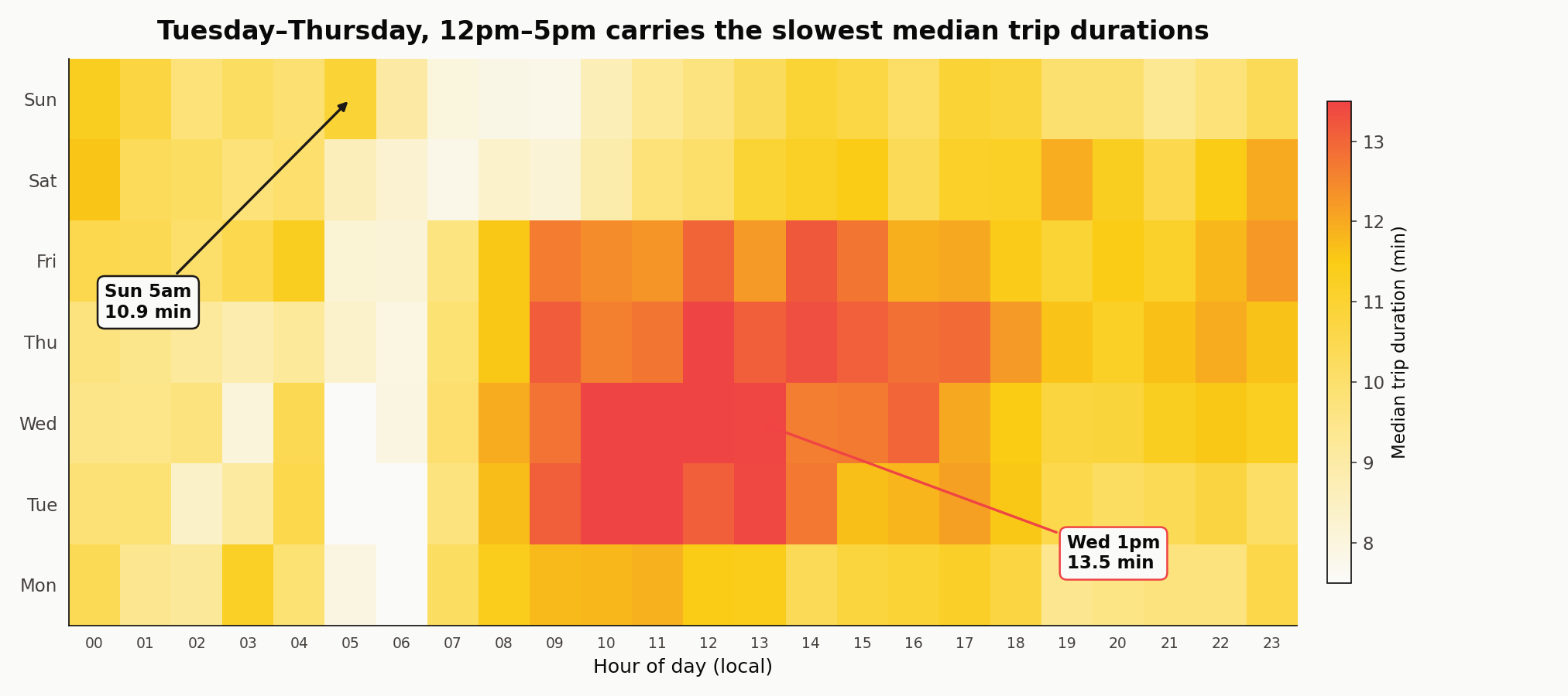
The slow hours cluster
Wednesday 1pm medians 13.5 minutes. Sunday 5am medians 10.9 minutes — long for the hour because the 211 Sunday-5am rides in the sample are disproportionately long-haul post-nightlife trips out of Manhattan, not the short commuter hops that dominate Tuesday 6am. Tuesday 6am medians 7.3 minutes by contrast. Any model that ignores hour and weekday is leaving that six-minute spread on the floor.
The dataset
The Kaggle NYC Taxi Trip Duration mirror carries 1,458,644 trips with pickup and dropoff coordinates, pickup datetime, passenger count, vendor ID, and trip_duration in seconds. I filtered to rides between 60 seconds and two hours, coordinates inside the NYC bounding box, and Haversine distances between 0.1 and 80 km. That drops 1.5 percent of rows — mostly dropoffs mis-coded in the middle of the Atlantic or durations under a minute.
All modeling runs on a 150,000-row random sample. The full 1.44M gives a slightly lower RMSLE (about 0.32 versus 0.323) and takes an order of magnitude longer to train. The feature ranking is identical either way.
Where the pickups happen
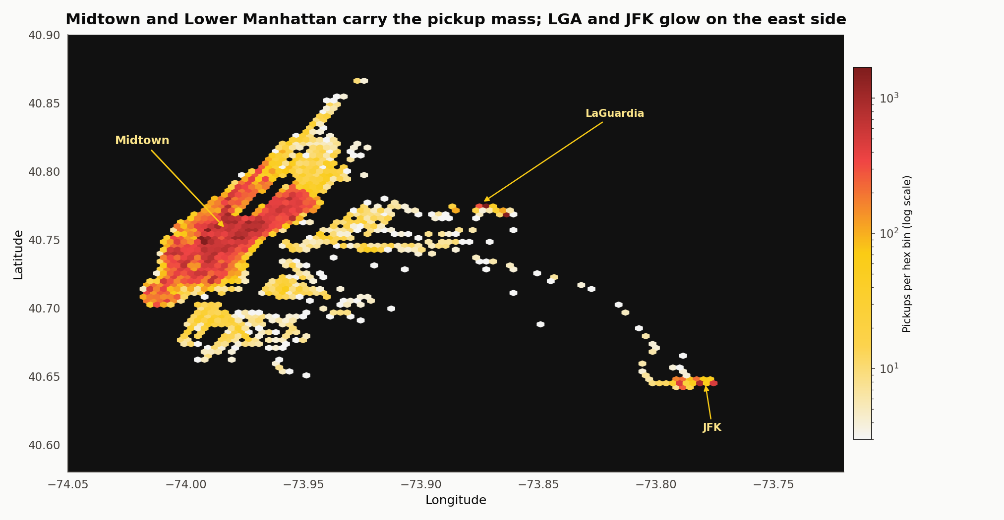
Midtown and Lower Manhattan carry the pickup mass. Brooklyn and Queens bands are thinner but visible. LaGuardia and JFK show up as small bright cells on the east side. Staten Island is nearly dark — yellow cabs don’t run there much, and the dataset does not include the outer-borough green cabs that would.
Duration by hour
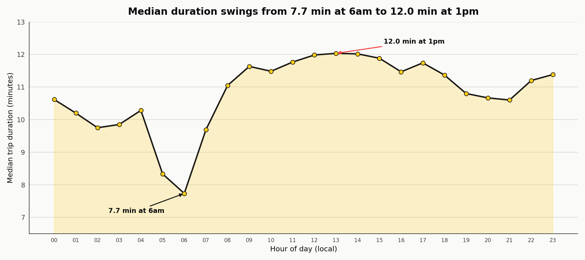
Median duration falls to 7.7 minutes at 6am and climbs to 12.0 minutes at 1pm. Morning rush runs 11.0 minutes at 8am, 11.6 at 9am, 11.5 at 10am, and 11.8 at 11am. The curve is a broad 11-to-12-minute plateau from 8am through 6pm rather than a sharp spike. A distance-only model sees none of this; it reads the same two coordinates and predicts the same duration regardless of when the trip happened.
Haversine versus Manhattan distance
| Two distances for the same trip. Haversine is the great-circle distance (what the crow flies) computed on a sphere: $d = 2R\arcsin\sqrt{\sin^2(\Delta\varphi/2) + \cos\varphi_1\cos\varphi_2\sin^2(\Delta\lambda/2)}$. Manhattan distance sums the latitude and longitude deltas independently: $d = | \Delta\varphi | \cdot 111 + | \Delta\lambda | \cdot 111\cos\varphi_1$. This is what the cab would drive if the grid forced every move to be north-south or east-west. The measured median ratio is 1.33, which says a typical trip covers about a third more ground than the straight-line estimate. The theoretical maximum for a perfectly aligned 45-degree grid is π/2, around 1.57. The real ratio sits in the middle because Manhattan’s grid is rotated about 29 degrees off true north and because real trips use diagonals like Broadway, bridges, and tunnels. |
Cyclic encoding of hour-of-day
Hour is cyclic. Passing the integer 0 through 23 to a linear model introduces a fake discontinuity at midnight: 1am and 11pm look 22 units apart when they are actually two hours apart on the clock. The textbook fix is a sin/cos pair, hour_sin = sin(2πh/24) and hour_cos = cos(2πh/24), which maps each hour to a point on the unit circle. Linear regressors, kernel methods, and neural nets need this. Tree-based models like XGBoost do not — they split on raw hour at any threshold they like and learn the wrap-around through interactions with other features. This project feeds the integer hour and still recovers a correct time signal, but the encoding matters the moment the model type changes.
Two models on the same split
Both models fit on an 80/20 split of log(duration + 1) with RMSLE as the validation loss. The baseline uses 300 trees at depth 5; the full model uses 800 trees at depth 7 with subsampling and column sampling.
| Model | Features | RMSLE | MAE (seconds) | R² |
|---|---|---|---|---|
| Distance only | 1 (Haversine) | 0.434 | 258.4 | 0.641 |
| Full | 10 (geo + time + distance) | 0.323 | 176.6 | 0.802 |
The naive model captures 64 percent of the log-duration variance on distance alone. That is more than most people expect, which is why this is a useful baseline rather than a straw man. The full model cuts RMSLE by 26 percent and MAE by 32 percent.
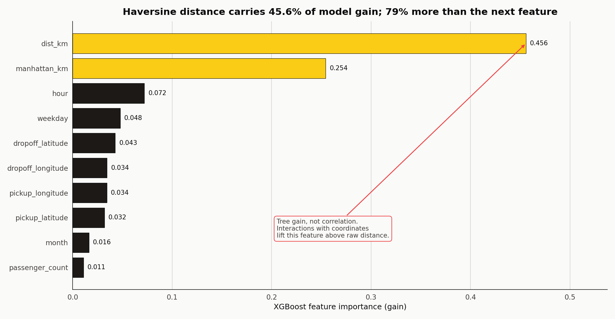
| Feature | Gain | Notes |
|---|---|---|
dist_km (Haversine) | 0.456 | Dominant predictor |
manhattan_km | 0.254 | Grid-correction signal |
hour | 0.072 | Temporal congestion |
weekday | 0.048 | Weekday vs weekend regime |
dropoff_latitude | 0.043 | Zone boundary |
dropoff_longitude | 0.034 | Zone boundary |
pickup_longitude | 0.034 | Zone boundary |
pickup_latitude | 0.032 | Zone boundary |
month | 0.016 | Seasonal drift |
passenger_count | 0.011 | Near noise |
Haversine carries 0.456 gain; Manhattan 0.254. That is the opposite of what you might expect if the grid intuition is doing the talking — Manhattan distance is closer to the driven distance, but Haversine takes more of the tree’s loss-reducing work once both are on the table. A leave-one-out check confirms the dependence runs that way: drop Manhattan and RMSLE worsens from 0.3227 to 0.3233. Drop Haversine and RMSLE worsens from 0.3227 to 0.3271. The two overlap, the tree picks Haversine first, and Manhattan refines.
The four coordinate columns together contribute 0.143 of gain — more than either distance feature alone. That is XGBoost acting as a regionaliser. Splits on latitude at 40.64 separate JFK trips from Midtown trips. Splits on longitude at -73.87 separate LaGuardia trips from Manhattan trips. The compound effect is that the model learns pickup and dropoff zones with no manual binning.
The duration surface morphs with time
Forty-eight frames. The left panel is median duration per pickup zone; the right panel is a clock and a weekday chip. Each hour plays twice (once for Wednesday, once for Sunday), so the same longitude and latitude get to show their two regimes. 8am Wednesday glows hot in Midtown and the Upper East Side. 8am Sunday is nearly uniform and two to three minutes faster everywhere. That is the temporal-spatial interaction the flat integer-hour feature has to carry, and it is why XGBoost’s ability to split on hour inside each coordinate branch matters more than the encoding choice.
An hour-by-hour pickup tour
Twenty-four frames. The Manhattan core stays dominant across every hour. What changes is the outer-borough mix (LaGuardia inbound pickups cluster at 7-9am, JFK outbound at 5-7pm) and the median trip duration, which moves from 7.7 minutes at 6am to 12.0 at 1pm.
What this isn’t
Not a live routing model. The dataset is from 2016. Manhattan traffic shifted materially with congestion pricing (January 2025) and the post-pandemic rebound. Anyone building a live duration estimator would want current data and weather covariates.
Not a leaderboard-winning submission. Top solutions on this competition use OSRM routing distances, hourly NOAA weather, and stacked ensembles. RMSLE 0.32 lands mid-pack. Winning entries reach 0.28.
Reproducibility note
Source code, notebook, and outputs in github.com/ndjstn/nyc-taxi-trip-duration. Dataset is the NYC.csv mirror of the Kaggle competition data (Kaggle, 2017).