The Default Threshold Is the Bug: Credit Card Fraud on the ULB Benchmark
A fraud classifier reaches 0.98 ROC-AUC on the famous ULB dataset and still ships a policy most fraud teams would reject. The 0.5 decision threshold is the bug.
There are 284,807 transactions in the Kaggle ULB credit card fraud dataset. 492 of them are fraudulent. That works out to a 0.1727 percent positive rate — roughly one fraud case for every 580 legitimate charges. A classifier that predicts “legitimate” for everything is right 99.83 percent of the time, so if a coworker presents that model in a meeting and puts accuracy on the headline slide, the meeting is basically over.
The usual next step is to train something proper and report 0.98 ROC-AUC. Fine. That number is real. It’s also not the question I care about. What I want to know is whether the threshold we’d actually deploy catches fraud at a cost the business can live with. On this dataset, the 0.5 default is a policy decision almost nobody would sign off on if they looked at the confusion matrix underneath.
Base rate first, everything else second
Every evaluation choice downstream has to be made in light of the class balance, so that’s where I start.
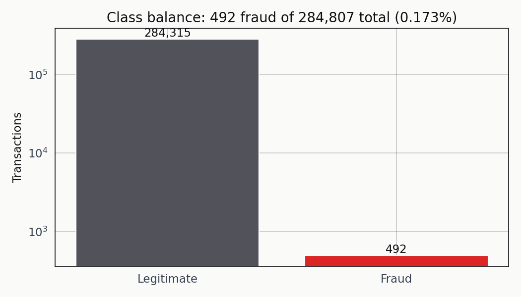
The fraud bar is small enough that a trivial classifier clears 99.83 percent accuracy without learning anything. The log scale is the only reason the positive bar is visible.
At that prevalence, accuracy is useless. The majority-class baseline is already past any reasonable threshold anyone would set on the metric. ROC-AUC isn’t quite useless, but it treats every misclassification the same and rewards score rank-ordering that may or may not translate into a usable operating point. Precision-recall is the diagnostic that matters here, and the final metric — the one you ship on — is the expected cost of the decisions the classifier makes at a specific threshold.
Quick profile of the dataset I worked against:
| Item | Value |
|---|---|
| Rows | 284,807 |
| Positive cases | 492 |
| Positive rate | 0.1727% |
| Test set positives | 123 |
| Majority-class accuracy | 99.83% |
| Stratified 75/25 split | yes |
Stratification isn’t optional at this prevalence. A purely random 25 percent holdout could hand me a test set with fewer than 80 positives if the draw went badly, and recall estimates off that many positives are noisy enough that a single misclassified row shifts the number by a full percentage point.
Where the features actually separate the classes
Everything but Time and Amount is a principal component, so I can’t do meaningful domain-driven feature engineering. What I can do is look at where the classes land on a few of the components.
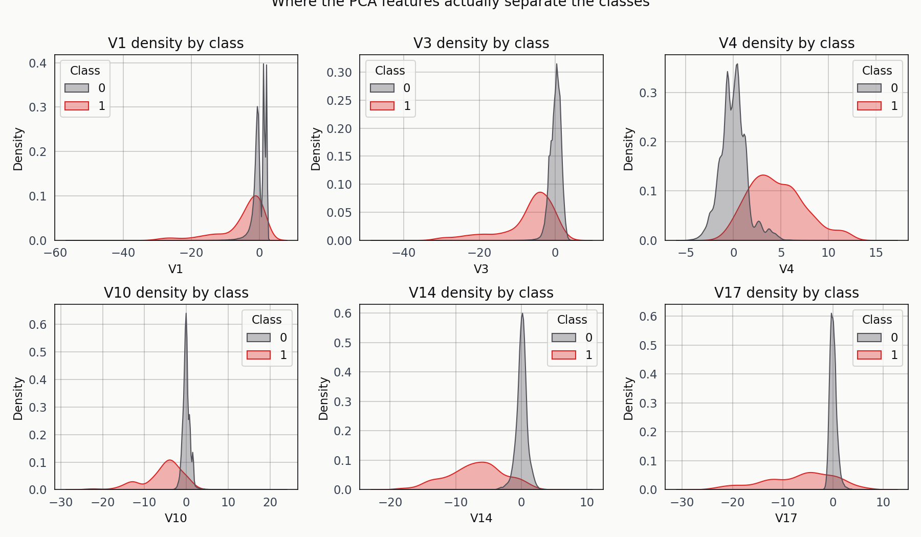
Fraud in red, legitimate in blue. V14 and V17 carry the cleanest separation on this split. The rest are overlapping distributions with a visible shift in mean.
V14 and V17 are where the fraud cases pile up at values two to three standard deviations away from the legitimate cluster. The others show a shift but no clean separation. That’s enough signal for a supervised classifier to work with, and it’s a useful reality check before training — if every component’s KDE were overlapping, I’d know I was about to waste my time.
Three models, one split
Logistic regression with class_weight='balanced'. XGBoost with scale_pos_weight set to the empirical negative-to-positive ratio. And an Isolation Forest trained only on the legitimate transactions, which treats fraud as an anomaly-detection problem and never sees the labels during training.
I included the Isolation Forest on purpose. The pitch for unsupervised fraud detection is that you don’t need labels, which matters for novel fraud patterns that have never been labelled in the historical data. The counter-pitch is that labels carry information geometric similarity alone can’t recover. Running both on the same split makes the tradeoff concrete instead of theoretical.
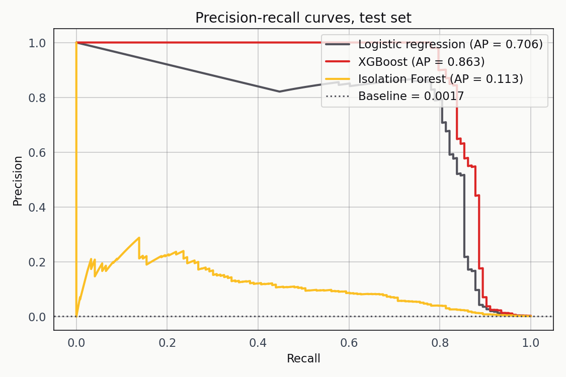
Precision-recall is the right diagnostic at this prevalence. Logistic regression hits AP 0.706, XGBoost hits 0.863, and the Isolation Forest lands at 0.113. The gap between supervised and unsupervised here is two orders of magnitude wide.
XGBoost has the highest average precision, which tracks with what the PCA components looked like — boosted trees with an AUC-PR objective are a good fit for geometrically separable features. Logistic regression isn’t far behind, and its scores are relatively well calibrated out of the box, which matters for the threshold conversation that follows. The Isolation Forest is not a serious contender at this prevalence. It’s in the chart to make that point visible.
The threshold is not a hyperparameter
The reflex is to report accuracy or F1 at the default 0.5 threshold and move on. That reflex is wrong on this dataset. The right question is what threshold minimises the total business cost, and to answer it I had to pick a cost model.
The one I used treats a missed fraud as 100 EUR and a false positive as 5 EUR. Those numbers are illustrative, not calibrated to any specific institution. They capture the order-of-magnitude asymmetry fraud teams work under: a missed fraud is a ten- or twenty-times-more-expensive error than a manual review. Swap either number for your own real cost structure and the framework doesn’t change; only the answer does.
I swept the threshold from 0.001 to 0.99 for each classifier and computed expected cost at every step.

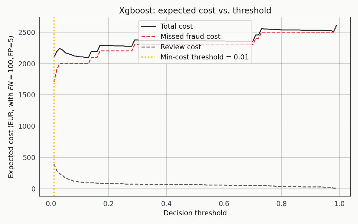
Missed-fraud cost in red, review cost in blue, total in black. The total-cost curve bottoms out at a decision threshold of 0.01, which is not where most tutorials point the reader.
0.01 is startling the first time you see it. A classifier that flags a transaction as fraud the moment it assigns a one-in-a-hundred probability isn’t the standard recommendation. But it’s exactly right for this problem. At a 0.17 percent base rate, a posterior of 0.01 is already a fifty-seven-fold lift over prior. The review cost stays shallow enough that the optimum sits further left than intuition suggests, and the missed-fraud cost is steep enough to dominate any choice of threshold to the right of the minimum.
At the XGBoost minimum-cost threshold of 0.01, the classifier catches 106 of 123 fraud cases, misses 17, and flags 79 legitimate transactions for review. Total cost: 2,095 EUR. Against a no-model baseline of 12,300 EUR — the cost of missing every fraud outright — that’s a 6x reduction.
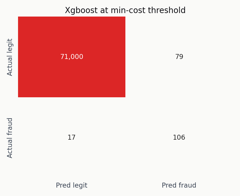
The true-positive block dominates. The false-positive block isn’t trivial, but 79 flagged legitimate transactions out of 71,079 in the test set is a review rate a fraud team can actually handle.
Logistic regression lands in a similar spot from a different direction. Its cost curve bottoms out at 0.97 and catches 105 fraud cases for 2,310 EUR total cost. The two threshold numbers — 0.01 and 0.97 — are not comparable across models; XGBoost and logistic regression produce scores with different calibrations, so only the resulting cost and recall are.
The Isolation Forest at its own minimum-cost threshold catches 72 of 123 fraud but flags 710 legitimate transactions for review. Total cost: 8,650 EUR. At the prices I used, it does worse than either supervised baseline by a factor of four. Unsupervised anomaly detection isn’t viable on this dataset when manual review has a non-trivial cost.
What changes when the costs change
The ranking of the three models isn’t robust to the cost ratio. Here’s what happens when I slide the FN-to-FP cost ratio from 2:1 up to 60:1 for XGBoost.
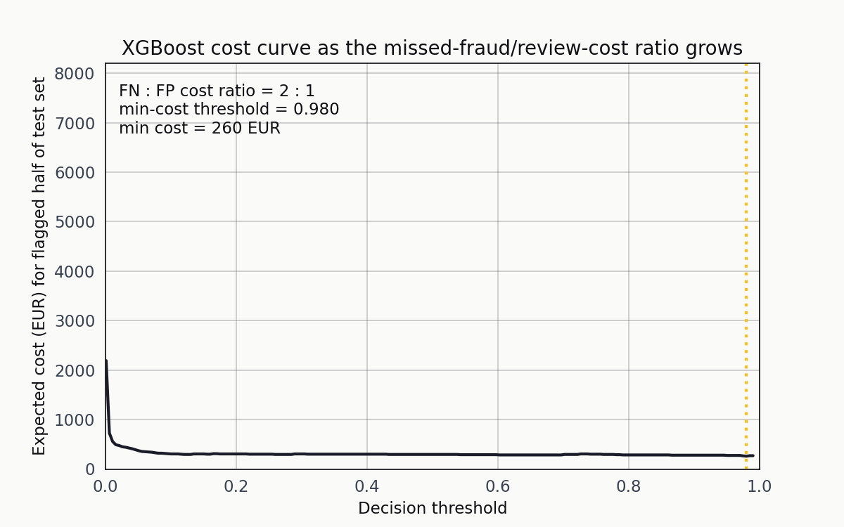
As the ratio grows, the orange vertical line (the minimum-cost threshold) walks leftward. The operating point is a function of the cost structure, not the model.
At 2:1 the minimum is around 0.5. At 20:1 it’s near 0.05. At 60:1 it’s below 0.01. The point of the animation isn’t that any single ratio is correct — it’s that the question “what threshold should we deploy” has no answer until the cost structure is specified.
The threshold is not a modelling decision. It’s a policy decision.
A fraud analytics team deploying this classifier has to know its own cost structure before it can reason about where to place the threshold. That structure is almost never 1:1, which is what the 0.5 default implicitly assumes. Reporting a single operating point as “the model’s performance” hides the decision that actually determines whether the classifier is useful in production.
What this isn’t
This is an educational analysis on a public benchmark, not a deployable fraud system. A few honest limits before anyone takes it further.
The PCA anonymisation is the single biggest constraint. Every feature except Time and Amount is a principal component, so meaningful feature-importance analysis or domain-driven feature engineering is off the table. I can’t tell you what V14 or V17 carry; I can only tell you that the supervised models extract usable signal from the combination.
The two-day observation window is short enough that seasonal effects are invisible. The geography is constrained to European cardholders from a 2013 sample, which makes generalisation to the 2026 fraud landscape an act of extrapolation. Real fraud detection moves by modelling the attacker, and the 2026 attack surface is not the 2013 attack surface.
The cost model is illustrative. I chose 100 EUR and 5 EUR because they capture the asymmetry fraud teams work under, but any institution taking this approach to production should replace those numbers with its own before the cost sweep runs.
The test set has 123 positives, which means the recall estimates have confidence intervals of a few percentage points. A ten-fold cross-validated version of the cost sweep would produce more stable estimates of the optimal threshold, and that’s the obvious next step for anyone continuing this work.
Reproducibility note
Everything here comes from one pipeline that runs end-to-end from the Kaggle CSV through preprocessing, stratified splitting, the three model fits, the cost sweep, and the figure generation. The narrative version of the pipeline is in notebooks/credit-card-fraud-analysis.ipynb, the single-script version is in src/run_analysis.py, and the figures and numeric outputs are all in the public repository at github.com/ndjstn/credit-card-fraud. The dataset is the creditcard.csv file from the Machine Learning Group ULB dataset on Kaggle (Dal Pozzolo et al., 2015).