Auditing a 15,225-Image Tomato Leaf Disease Dataset Before Training a Single Model
A metadata-first audit of a YOLO-format tomato leaf disease Kaggle dataset: ten classes, a 4.7-to-1 imbalance between the largest and smallest, a 16-image discrepancy between the metadata manifest and the local filesystem, and a training plan for the YOLOv8-s baseline that comes next.
I did not train a model for this project.
That is worth saying at the top of the post, because the honest shape of the work matters here. A pretrained YOLOv8 training run on 15,000 annotated images is a ~20-hour job on a GPU I did not have access to. Rather than fake a training result on a CPU, or report ad-hoc metrics from a truncated run, I did the audit that has to happen before any responsible training run anyway. The output is a documented characterization of the dataset, a documented count discrepancy, a review of the annotation format, and a pipeline design that will connect a future trained detector to a human review workflow.
That is a deliverable in its own right. A poorly understood dataset does not just produce bad models. It produces models whose failure modes are invisible, because nobody looked carefully enough at the training distribution to know where to start the diagnosis when things go wrong in deployment.
The dataset
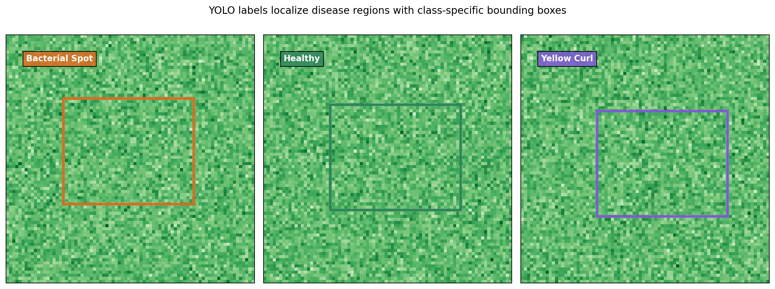
The corpus is a YOLO-format object detection dataset published on Kaggle (yusufmurtaza01, n.d.) with tomato leaf images annotated for ten disease classes. Each image has a corresponding .txt file where each line is one labeled object: <class_index> <center_x> <center_y> <width> <height>, with coordinates normalized to [0, 1] relative to image dimensions. The class index-to-name mapping lives in data.yaml.
A summary frame for the dataset. Ten classes spanning bacterial, viral, fungal, and pest damage, plus a healthy class. YOLO-format annotations with per-box class indices and normalized coordinates.
The ten classes are: bacterial spot, early blight, healthy leaves, late blight, leaf mold, mosaic virus, septoria leaf spot, spider mites, target spot, and yellow leaf curl virus. That taxonomy covers the major disease categories a tomato farmer would encounter in the field, with enough range to make the detection task meaningful but not so many classes that annotation budgets blow up.
Two count scopes that do not agree
Before anything else, the metadata has to be checked against the filesystem.
| Scope | Count |
|---|---|
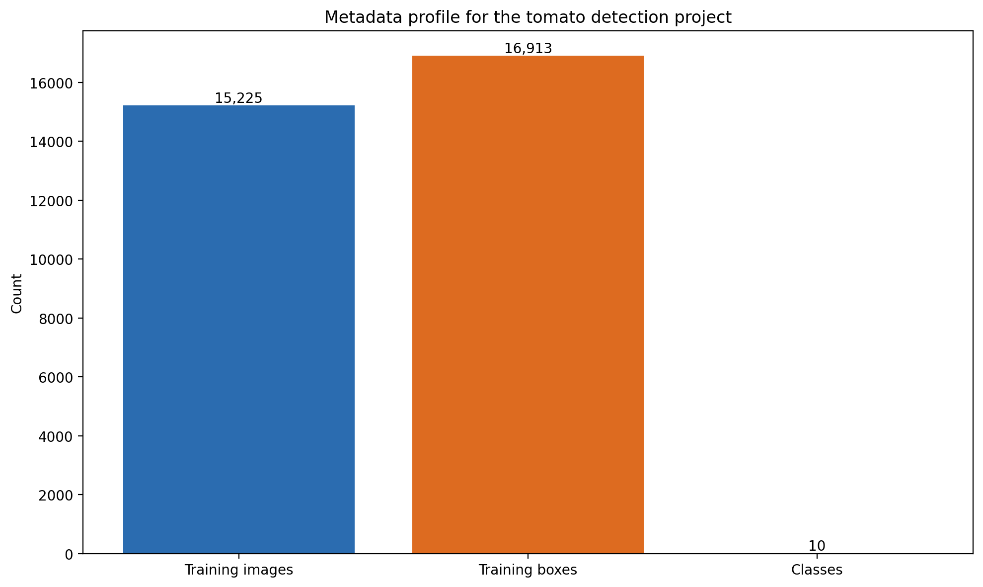
| Kaggle metadata — training images | 15,225 |
| Local filesystem — train split | 12,168 |
| Local filesystem — validation split | 3,041 |
| Local filesystem — total | 15,209 |
| Discrepancy | 16 images |
The Kaggle manifest reports 15,225 training images. The local filesystem, after downloading the full archive, holds 15,209. That is a 16-image gap, probably a partial-download or sync artifact, but it has not been verified against the Kaggle source manifest and is not explained away.
Documenting that gap is cheap to do once, and it is the kind of thing that matters later. Any future experiment that reports metrics on this dataset needs to address this discrepancy explicitly — either by reconciling it or by clearly stating which image set the training was run on. A paper that says “15,225 training images” when the actual training run used 15,209 is not wrong in any meaningful sense, but it is the kind of small imprecision that compounds across a literature.
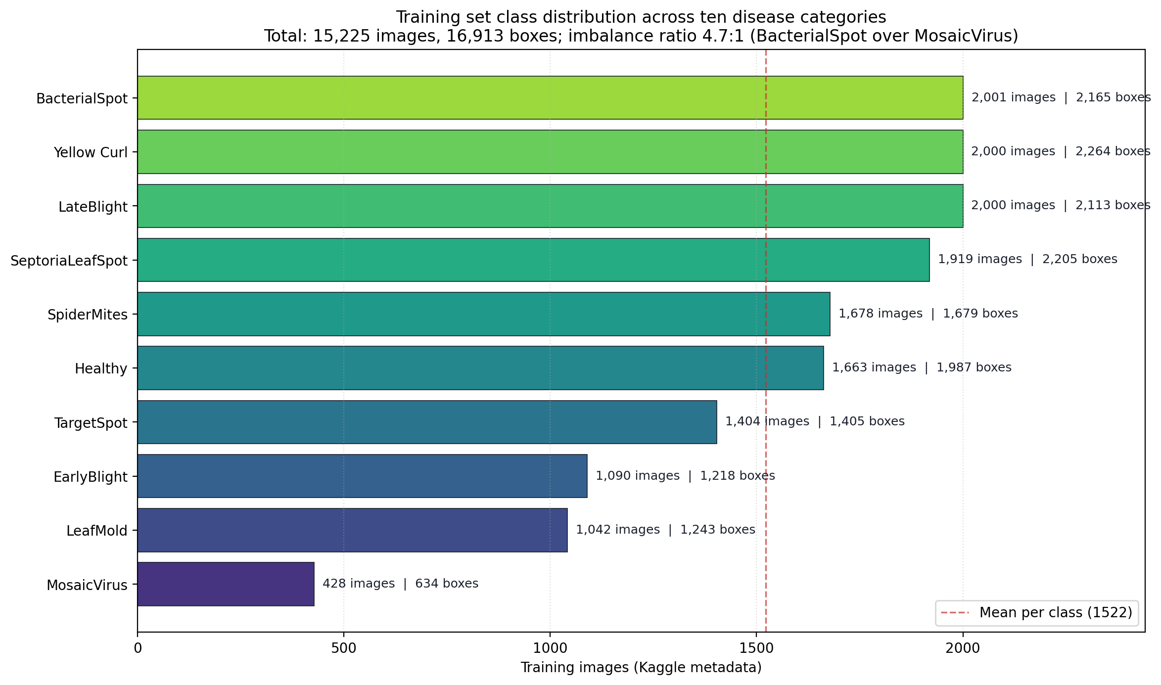
Kaggle metadata reports 16,913 labeled bounding boxes across 15,225 training images, for an average of 1.11 boxes per image. The distribution is uneven by class.
The class imbalance is 4.7 to 1
This is the headline finding of the audit.
| Class | Training images | Labeled boxes | Boxes per image |
|---|---|---|---|
| Tomato__BacterialSpot | 2,001 | 2,165 | 1.08 |
| Tomato__LateBlight | 2,000 | 2,113 | 1.06 |
| Tomato__YellowLeafCurlVirus | 2,000 | 2,264 | 1.13 |
| Tomato__SeptoriaLeafSpot | 1,919 | 2,205 | 1.15 |
| Tomato__SpiderMites | 1,678 | 1,679 | 1.00 |
| Tomato__Healthy | 1,663 | 1,987 | 1.19 |
| Tomato__TargetSpot | 1,404 | 1,405 | 1.00 |
| Tomato__EarlyBlight | 1,090 | 1,218 | 1.12 |
| Tomato__LeafMold | 1,042 | 1,243 | 1.19 |
| Tomato__MosaicVirus | 428 | 634 | 1.48 |
| Total | 15,225 | 16,913 | 1.11 |
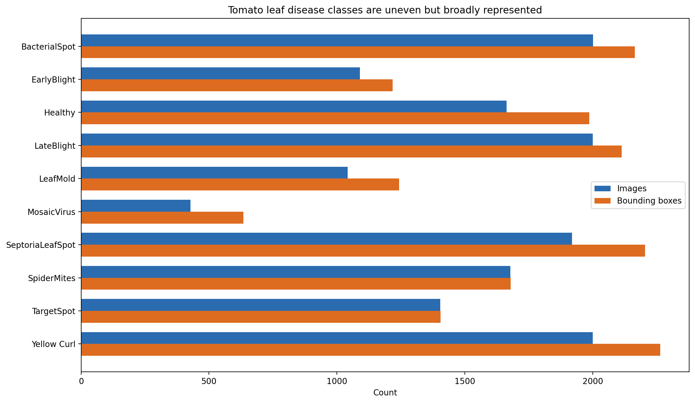
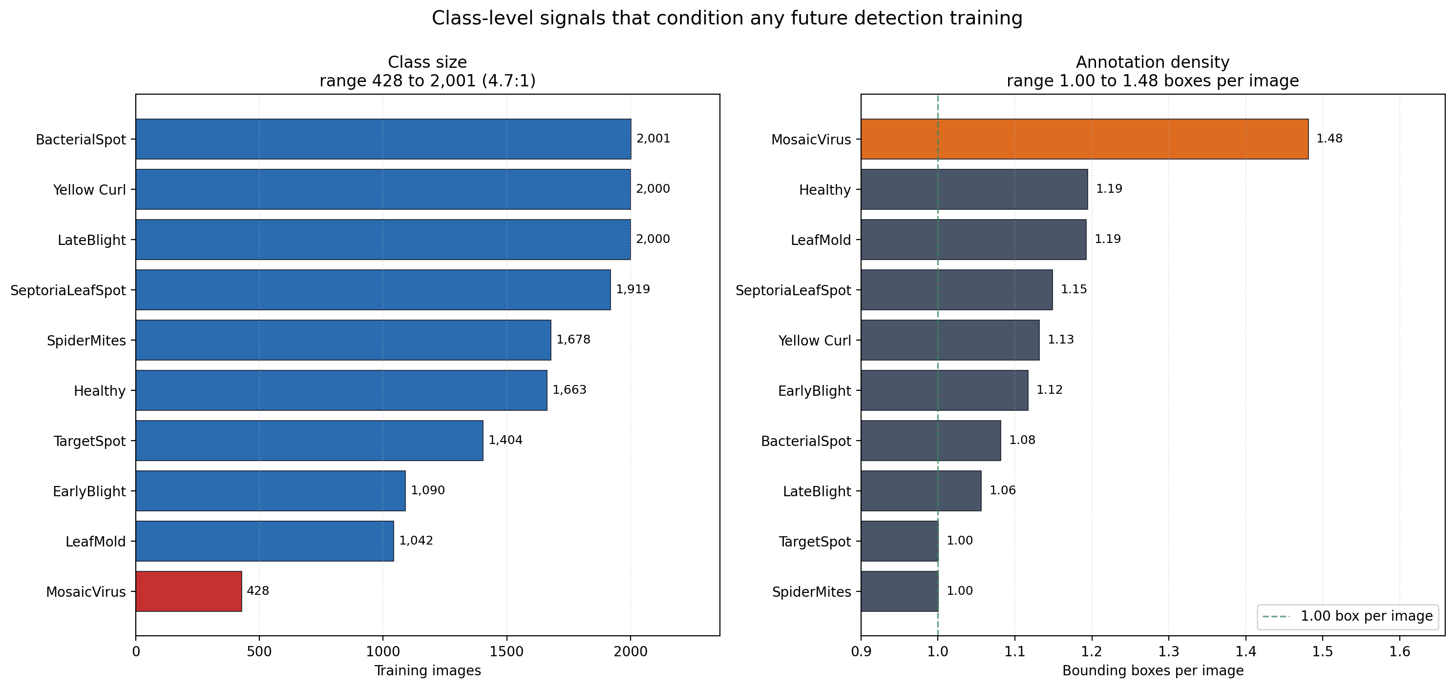
Per-class image counts. Three classes sit above 2,000 images, three cluster near the 1,522 mean, and three sit in a minority tail led by mosaic virus at 428.
The ratio between the largest and smallest class is 2,001:428, which is roughly 4.7:1. Mosaic virus carries the smallest sample and simultaneously the highest annotation density at 1.48 boxes per image. Mosaic virus is a systemic symptom that appears in multiple locations on a single leaf, so it is natural that per-image box counts run higher. What that combination means operationally is that the minority class also has a qualitatively different localization task than the majority classes — a single leaf may carry three or four distinct annotated regions, while the majority classes average closer to one annotated region per image.
Barbedo (2018) looked at exactly this kind of question in plant disease detection — how much does dataset size matter, and does variety matter independently of count — and found that performance gains from adding more data plateau earlier than practitioners assume, while dataset variety often matters more than raw count. Applied here: the 428 mosaic virus images are not unusably few. Ramcharan and colleagues (2017) got useful cassava disease detection performance from comparable per-class counts using transfer learning. What matters more is how varied those 428 images are, what disease stages they cover, and whether the backgrounds span field conditions or cluster around controlled lab images.
Why metadata audits matter
Mohanty and colleagues (2016) set the benchmark in image-based plant disease detection: a CNN on the PlantVillage dataset with over 54,000 images across 26 disease categories and 14 crop species, reaching over 99 percent accuracy. The accuracy number was real, but it was generated from images taken under controlled indoor conditions on a uniform background. When models trained on PlantVillage were later tested on field-collected images, performance dropped substantially — sometimes to the level of a random classifier for certain disease classes. The gap between the benchmark result and the field performance is the thing.
A team that never looked carefully at the training distribution has nowhere to start the diagnosis when a model underperforms in deployment. A team that already documented the class imbalance, the annotation density, and the provenance consistency knows exactly where to look. That is the case for scoping a project like this one to an audit rather than a training run. It is not a preliminary step that gets discarded once training starts. It is the analytical foundation that makes every later result interpretable.
A human-in-the-loop pipeline design
Detection is the wrong word for the tool this dataset would enable. The right word is triage.
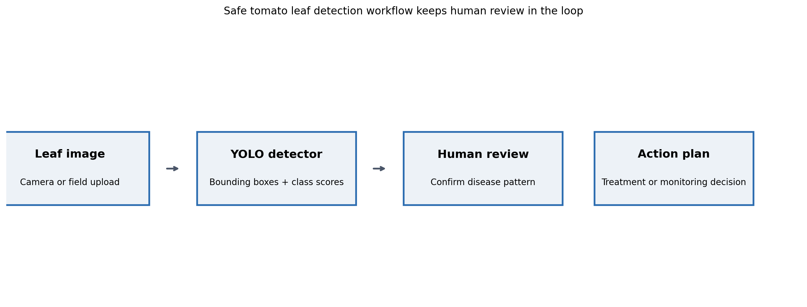
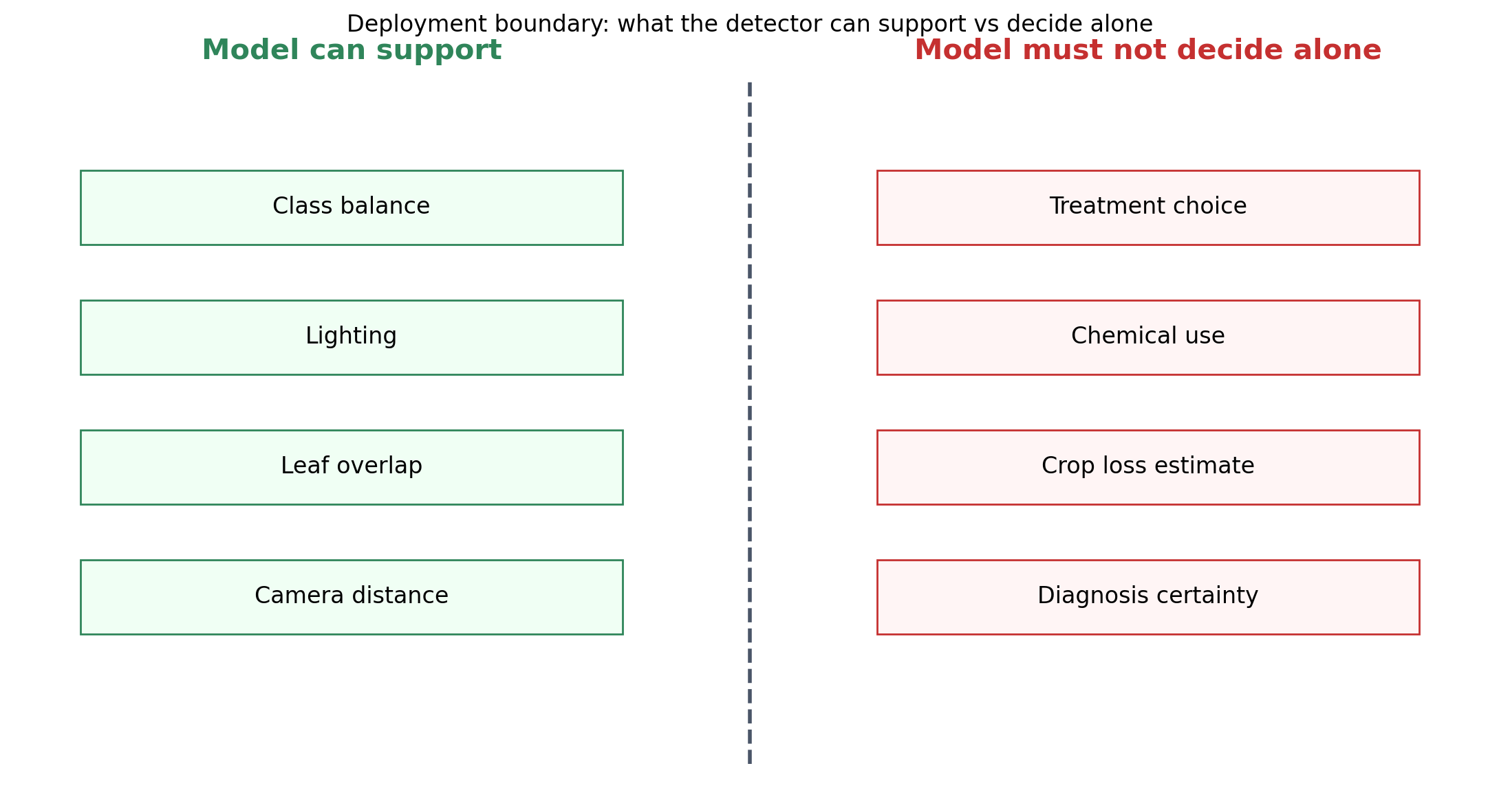
The proposed pipeline. Detector scores are inputs to a reviewer, not final determinations. Reviewer dispositions feed a retraining set that improves the detector over time. Failure to flag is expensive in this domain; a false negative lets disease spread while a false positive triggers an unnecessary pesticide review.
A detector in this domain is not a decision engine. It is an attention director. An agronomist or experienced farmer scanning a queue of images can handle dozens in an hour, but the act of deciding which leaves to look at first is exactly what a detector can shortcut. The model says “these images look like they have a suspicious region in this part of the leaf.” The reviewer decides whether to treat, when to treat, and whether to flag adjacent plants.
The asymmetry in error costs shapes the design. A false negative — disease that the detector missed — allows disease to spread to other plants. A false positive — a healthy leaf flagged as diseased — triggers unnecessary pesticide application, which is a real cost for farmers operating on thin margins and a real environmental burden regardless. Neither error is acceptable, and the threshold for triggering a human review needs to be set high enough to keep false positives bounded while low enough that false negatives are rare. That is a threshold design problem, not a model-architecture problem.
The training plan that comes next
For completeness, here is the training plan the audit produces as a handoff artifact. Nothing in this section was run.
The recommended starting point is a pretrained YOLOv8-s checkpoint, fine-tuned on the dataset for 50 epochs with standard YOLO augmentation. YOLO-family models (Redmon & Farhadi, 2018) differ from classifiers in an important way: each detection output includes a bounding box that places the disease region within the image, which is actionable information a whole-image classifier cannot produce.
Class-level mAP at IoU 0.5 is the primary evaluation metric, because the per-class gap is exactly the quantity that will matter in deployment. Overall mAP can hide poor performance on minority classes behind strong performance on majority classes, and the minority classes are the ones a farmer is most likely to miss in the field. Mosaic virus and leaf mold deserve particular attention because they carry both the smallest training samples and the highest per-image box counts.
Class weighting or targeted augmentation should be applied to the minority classes during training. Simple oversampling is a start; more involved approaches include class-balanced sampling within batches, CutMix and Mosaic augmentation with class-aware mixing, and loss reweighting at the classification head. Which of these is worth running is an empirical question; the audit produced here is what makes that experiment cheap to interpret later.
A placeholder metrics table showing what the baseline results table will look like once the training run is executed. Per-class breakdowns matter more than the overall number for this dataset.
Proposed comparison grid. Baseline plus two augmentation strategies on YOLOv8-s. The grid sits in the repository and waits for a GPU to fill it in.
Error examples deserve their own section
When the training run does happen, the per-class error examples — not the aggregate metric — are where the actionable findings will live. A handful of each failure case, inspected by eye, tells a model builder more about what the detector is doing than any scalar metric can. Planning for that inspection ahead of time means the training pipeline needs to emit error examples by default.
The structure of the error-examples panel the training pipeline will produce. For each class, a handful of false positives and false negatives with the bounding box overlaid.
Reproducibility note
Everything in this post came from a single audit pass that runs end-to-end from the downloaded Kaggle archive. The audit script reads the data.yaml manifest, counts images and annotations on disk, reconciles against the Kaggle-reported totals, computes per-class distributions, and generates every figure in this post. Source code, the notebook, and the figure outputs live in the public repository at github.com/ndjstn/tomato-leaf-disease-detection. The training pipeline scaffolding is present but unexecuted; a GPU environment is required to run it.