The Mental Model That Made Neural Networks Finally Click for Me
Most explanations of neural networks start in the wrong place. This is the mental model that finally made layers, weights, activations, and backprop feel concrete to me.
The first few times I tried to learn neural networks, I had the same reaction I have to a lot of bad technical writing: I could tell the author knew what they were talking about, and I could also tell they were making the subject harder than it had to be.
The explanations kept starting with the nouns: neuron, weight, bias, activation function, hidden layer, backpropagation. Those are useful words eventually, but they did not answer the question I was stuck on: what job is the system actually doing?
I did not need more vocabulary. I needed a working picture. Once I had one, the terminology stopped feeling like a pile of disconnected labels and started feeling like names for parts inside a machine.
The picture that finally worked for me was this:
A neural network is a layered scoring system.
Each layer takes in signals, scores what seems important, reshapes the representation a little, and hands something more useful to the next layer.
That is not the formal definition. It is just the version I wish I had started with, because it gives the pieces somewhere to sit.
The rest of this post is basically the explanation I wish I had been given earlier.
Most explanations start in the wrong place
The usual beginner explanation goes something like this: here are the components, here are the names, here is a diagram, and eventually it will all make sense.
I don’t think that is a very good way to teach the subject. It front-loads the least helpful part.
If you start by memorizing terms, you wind up with the shape of the topic but not the feel of it. You can point at a diagram and say “that’s a hidden layer,” but that is very different from being able to say what the layer is actually contributing.
The “job-first” view works better because it gives the system a purpose before it gives the system labels.
A neural network is trying to map inputs to outputs.
The input might be pixels, text, rows in a spreadsheet, or some messy real-world signal. The output might be a class label, a probability, a score, a forecast, or some generated sequence.
Everything inside the model exists to improve that mapping.
If you want the compact mathematical version, it is just this:
\[\hat{y} = f_{\theta}(x)\]Input $x$ goes in, prediction $\hat{y}$ comes out, and the parameters $\theta$ are what training keeps adjusting. That compact view is the one open deep-learning textbooks usually start from (Goodfellow et al., 2016).
If you want one more layer of detail, you can think of $f_{\theta}$ as a composition of smaller transformations:
\[f_{\theta}(x) = g^{(L)}\!\left(g^{(L-1)}\!\left(\cdots g^{(1)}(x)\right)\right)\]The notation is doing useful work here. It shows the network as a chain of transformations, not a pile of mysterious parts.
That view scales. Two layers, twenty layers, two hundred layers—it is still the same basic pattern: take something in, transform it, pass it forward. After that clicked, the subject felt less like a collection of exceptions and more like one repeated idea.
- neuron: score local evidence. Does this pattern show up here?
- bias: move the trigger point. How much evidence is enough?
- activation: reshape the response. How hard should it fire?
- backprop: route correction backward. Who should change most?
Once I attached each label to a job, the rest of the topic got much easier to hold in my head.
What a neuron actually is
The word “neuron” does a lot of damage, honestly. It suggests biology, mystery, maybe some tiny synthetic brain cell doing something profound.
The underlying operation is much less dramatic.
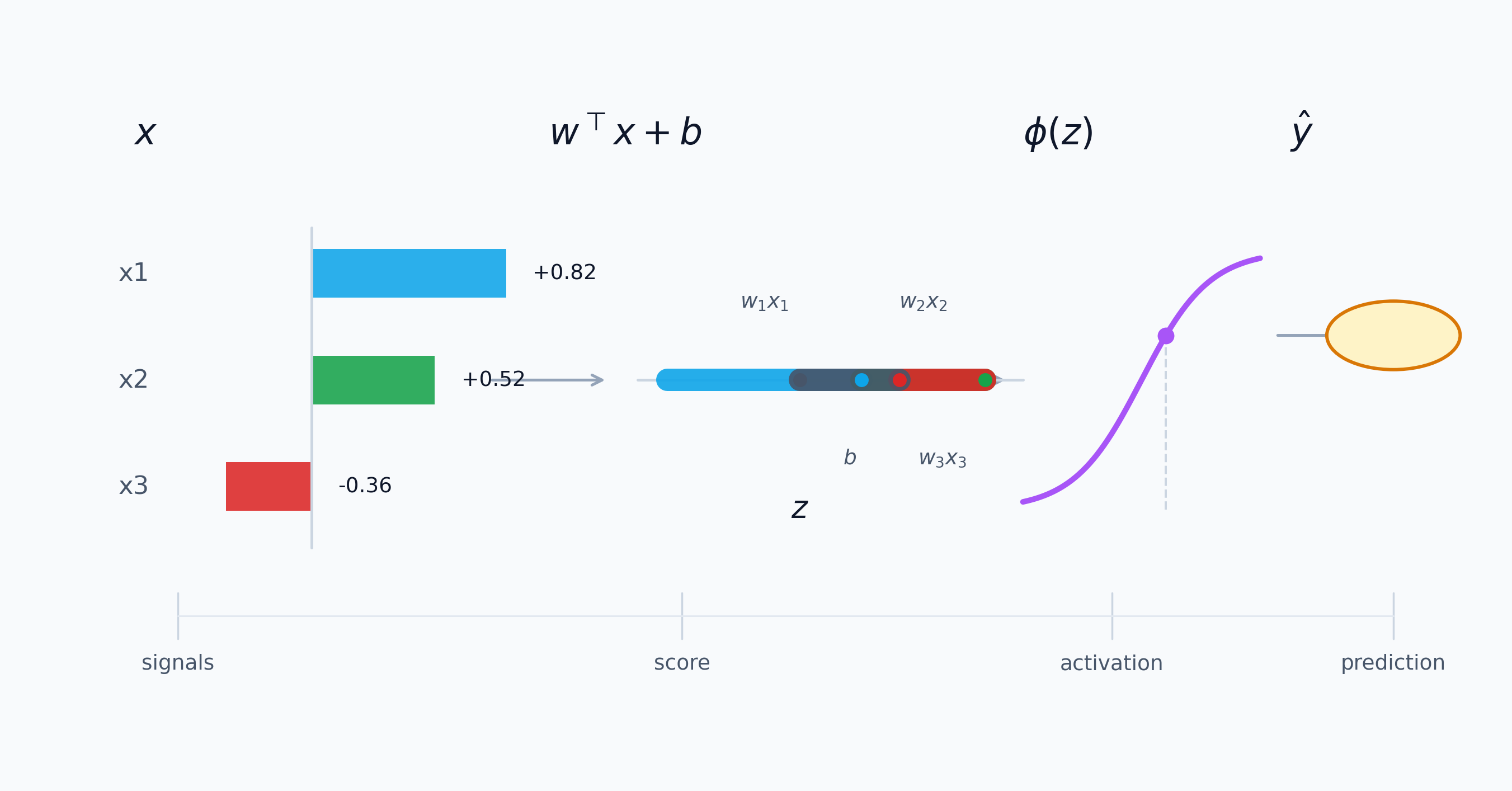
A neuron takes in numbers, weights them, adds a bias term, runs the result through an activation function, and passes the output onward.
Written compactly, that looks like this:
\[z = \sum_{i=1}^{n} w_i x_i + b, \qquad a = \phi(z)\]In modern machine-learning terms, this is the standard feedforward / perceptron view you see in open textbooks and course notes (Goodfellow et al., 2016; Google, n.d.-b).
The power does not come from one neuron doing something clever. It comes from running the same dumb little operation thousands of times until the combined effect becomes useful.
I think of neurons as scoring rules now. A neuron is not thinking. It is computing a weighted sum, shifting it with a bias, passing it through a nonlinearity, and sending the result forward.
Most of those scores are meaningless on their own. The value shows up when later units combine them into something the model can actually use. The brain metaphor gets in the way here. If you expect intelligence at the neuron level, you will be disappointed. If you expect simple operations compounding into capability, the whole system makes much more sense.
Illustrative values, same pattern: evidence comes in, gets combined into one score, then gets turned into a stronger or weaker response.
Neural networks became easier for me once I stopped looking for intelligence at the neuron level. It is cleaner to imagine tiny scoring operations building toward something useful.
Weights and biases do different jobs
Weights are where the model learns what to care about.
If two signals come into the same unit and one gets a large weight while the other gets a small one, that is the model saying, in effect, “this signal should count more than that one.”
Weights matter because they are the model’s learned preferences about influence. When training goes well, the model keeps adjusting those preferences until patterns that help the task get emphasized and patterns that don’t help get pushed down.
Biases are different.
Biases do not answer “what matters most?” They answer something closer to “how easy should it be for this unit to wake up and respond at all?”
That sounds minor until you realize how much flexibility it adds. A bias lets the model shift the point where a unit starts responding strongly. Without that shift, the model is more rigid than it needs to be.
The simplest way I can say it is this:
- weights control influence
- biases shift sensitivity
A useful way to see both jobs together is the linear score
\[s = w^\top x + b\]where the entries of $w$ decide how much each input contributes and $b$ shifts the score up or down before the activation ever sees it.
The quick sensitivity read is useful too:
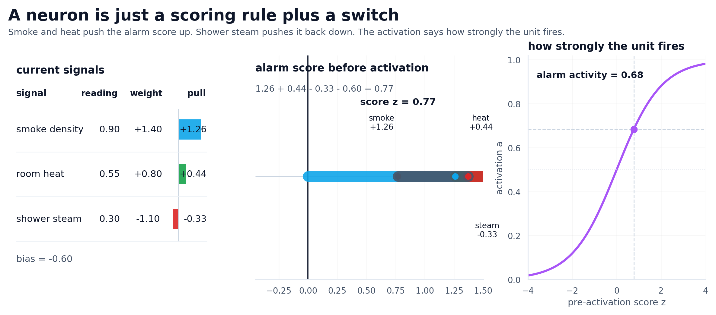
\[\frac{\partial s}{\partial x_i} = w_i, \qquad \frac{\partial s}{\partial b} = 1\]A useful weights-and-bias graphic should answer three plain questions: which inputs are active, which weights pull hardest, and where the bias moves the switch-on point. The standard nodes-and-hidden-layers framing is still useful here because it makes each input’s signed influence explicit (Google, n.d.-b).
That is not the full mathematical story, but it is the part I reach for when I want the intuition fast.
A thermostat is a cleaner example here than a classifier with mysterious embeddings. Imagine a smart heater deciding whether to kick on. A room that is well below target temperature should push the score up, so that signal gets a positive weight. Occupancy gets a positive weight too: if someone is home, the system should care more. Strong afternoon sun gets a negative weight because free warmth should pull the score back down.
Now hold that room state fixed. If the thermostat is in comfort mode, a less negative bias makes it easier for the same evidence to cross the line and turn the heat on. Switch to eco mode and the exact same room can stay off. Nothing about the room changed. Nothing about the weights changed. Only the baseline stubbornness changed.
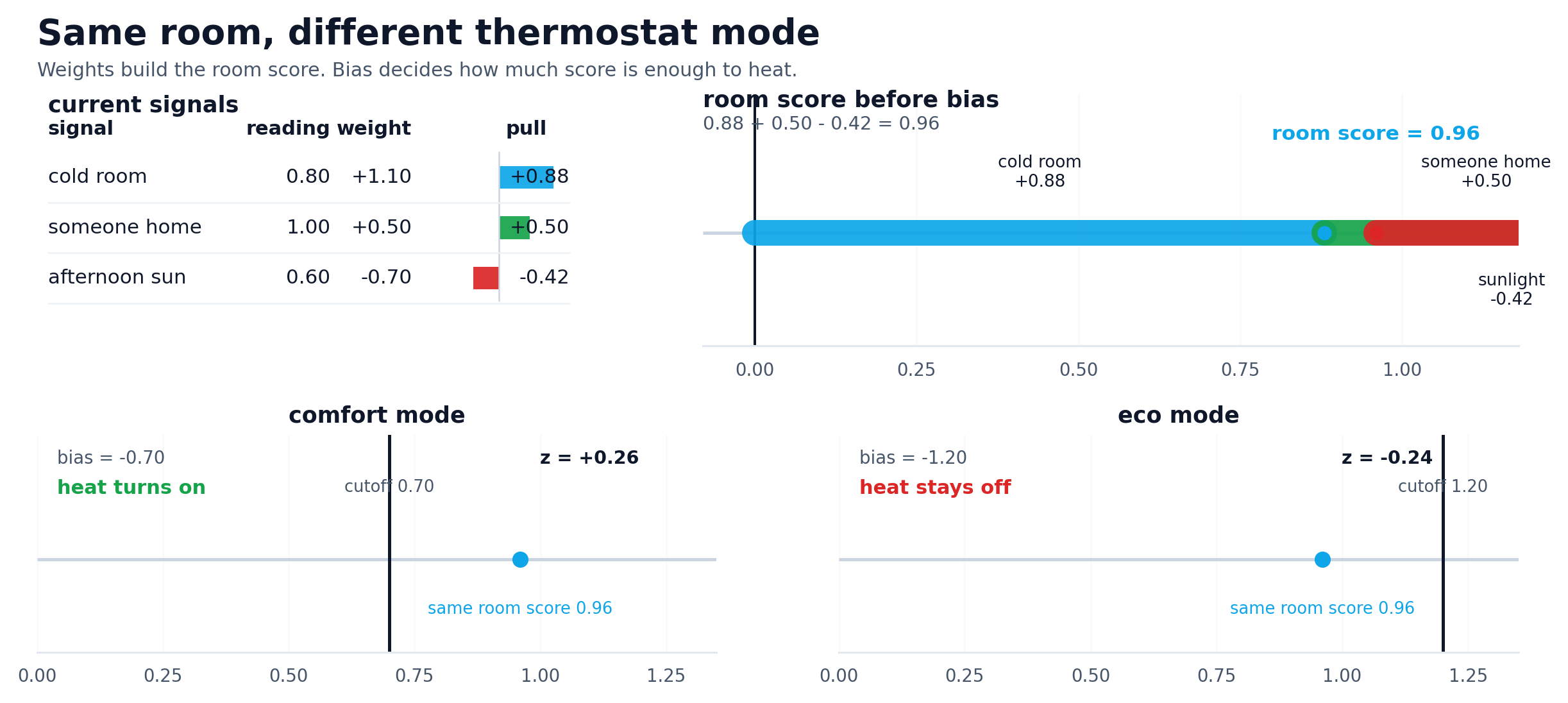
Illustrative thermostat values. The room state stays fixed; weights decide which signals push hardest, and bias decides how much evidence is enough.
On the left, one weight changes while the cutoff stays fixed. On the right, the cutoff moves while the room state stays fixed.
Activation is where things get interesting
Without activation functions, stacking layers is basically pointless. A linear transformation followed by another linear transformation is still just a linear transformation. You can make the network deeper, but you have not made it fundamentally more expressive.
That is the real job of activation functions. They break the straight-line behavior and let the model carve out decision boundaries that a purely linear stack never could. That is not a side detail. It is the reason deep networks are worth using in the first place.
In formula form, three common examples are:
\[\operatorname{ReLU}(x) = \max(0, x), \qquad \sigma(x) = \frac{1}{1 + e^{-x}}, \qquad \tanh(x) = \frac{e^x - e^{-x}}{e^x + e^{-x}}\]ReLU, Sigmoid, and Tanh are different curves with different tradeoffs, but the big idea is the same: they let the model respond in a way that is not just a simple linear rescaling of the input. The point of writing the formulas out is to make the shape change explicit; that is exactly why rectified units became so practically important in later deep models (Nair & Hinton, 2010; Google, n.d.-a).
That is what gives the network room to model XOR-like patterns, curved boundaries, and other structure a linear model simply cannot represent.
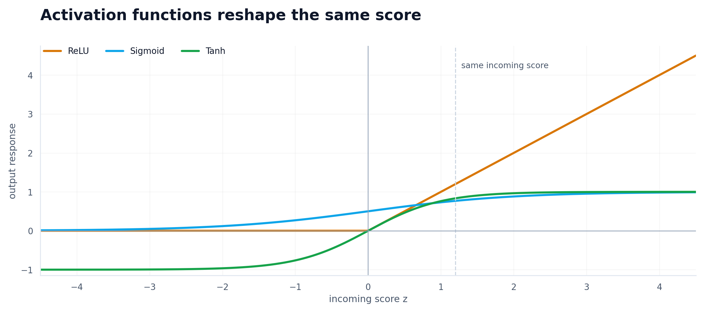
The exact curve changes, but the essential job stays the same: add non-linearity so the model can represent something more interesting than a straight line.
I treated activation functions like a vocabulary item for too long. They are much closer to the point where the model stops being a fancy linear map and starts becoming a useful learner.
Hidden layers are feature builders
The phrase “hidden layer” makes it sound like something secret is happening in there. Usually it is much more ordinary than that. A hidden layer is just an intermediate representation.
That is where a lot of the value in deep learning comes from. Each layer turns the input into a form that is easier for the next layer to use. That representation-building view is one of the core ideas behind modern deep learning more broadly (Goodfellow et al., 2016).
Early transformations often react to simpler patterns. Later transformations can combine those simpler patterns into more meaningful structures.
For images, that might mean edges before shapes, and shapes before object parts.
For text, that might mean local phrasing before broader semantic patterns.
For tabular data, it might mean combinations of variables that would have been annoying to hand-engineer.
The point is not that “depth is smart.” The point is that depth gives the model room to compose simpler signals into better features.
That composition usually looks something like this:
\[h^{(1)} = \phi\!\left(W^{(1)} x + b^{(1)}\right), \qquad h^{(2)} = \phi\!\left(W^{(2)} h^{(1)} + b^{(2)}\right)\]Each new layer is not starting from scratch. It is transforming the representation produced by the previous one.
The figure below uses a tiny learned network on synthetic two-moons data, then asks a simple question at each stage: if you freeze that representation, how well can a straight line separate the classes? That makes the phrase “better representation” visible instead of just saying it.
That shift made hidden layers feel less mystical. I stopped thinking, “there are magic layers in the middle,” and started thinking, “the model is trying to build a better internal representation before it makes a decision.”
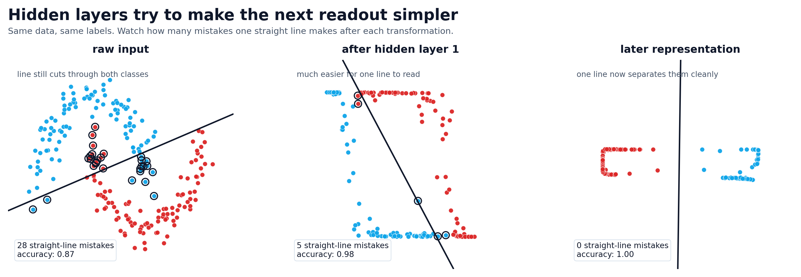
The same points become easier for a straight-line classifier to separate as the hidden representation gets cleaner.
Backprop is just accountability
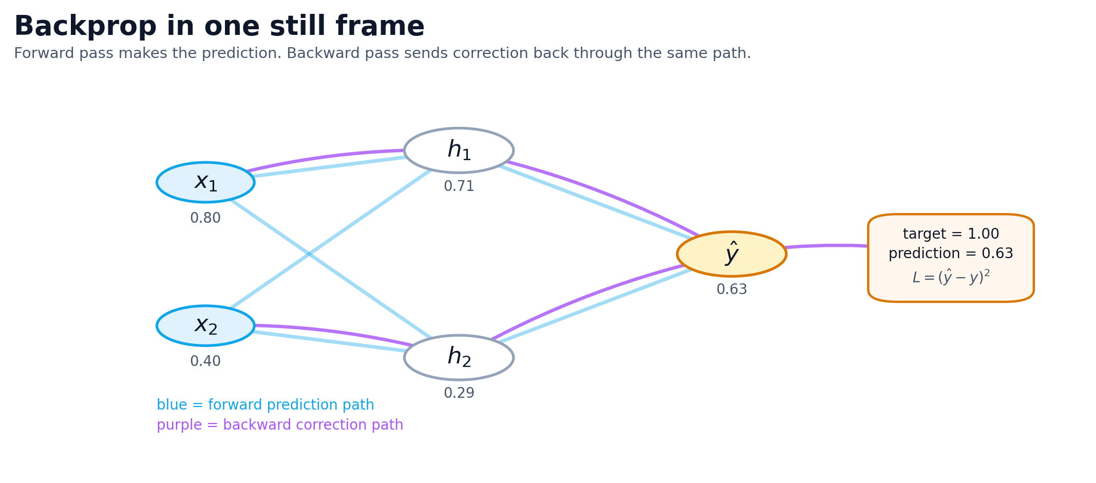
Backpropagation sounded intimidating to me for longer than it deserved to. The name makes it sound more exotic than the working idea.
The model makes a prediction. You measure how wrong it was. Then you push that error signal backward so the parameters that contributed to the miss can be adjusted.
What made backprop click for me was treating it like blame assignment. The model missed. The question is which parameters contributed to the miss, and by how much.
Backprop pushes the error backward through the graph so each weight gets a gradient telling it how its change would affect the loss. It is bookkeeping for repeated correction.
The training loop usually gets summarized with a loss function and an update rule:
\[L(\hat{y}, y) \qquad \text{and} \qquad W \leftarrow W - \eta \, \nabla_W L\]The loss says how wrong the prediction was. The gradient tells you how to move the weights. The learning rate $\eta$ controls how large a step you take.
If you want the “who gets the blame?” version in one line, it is the chain rule doing bookkeeping:
\[\frac{\partial L}{\partial w_i} = \frac{\partial L}{\partial \hat{y}} \cdot \frac{\partial \hat{y}}{\partial w_i}\]That equation is the chain rule in its most useful form: how sensitive the loss is to the prediction, multiplied by how sensitive the prediction is to a specific weight. That is the bookkeeping at the heart of backpropagation (Nielsen, 2015; Google, n.d.-c).
The biggest gradients mark the parts of the model that would change the loss most if adjusted.
Bad training runs usually stop looking mysterious once you treat them as broken correction loops. Maybe the gradients are weak. Maybe the learning rate is wrong. Maybe the labels are noisy. Maybe the model has more capacity than the data can support.
Once you frame the problem that way, debugging gets less theatrical and more mechanical. You start checking the loop instead of reaching for a new architecture name.
The checklist I use when a model is going sideways
When a model underperforms, I almost never start by reaching for a new architecture. I start with a plain checklist.
What is the model being asked to predict? Which signals should matter if the task is being learned correctly? Does the model have enough capacity to fit the pattern without memorizing noise? Is the training signal useful? Is this a model problem or a data problem?
That line of questioning has saved me more time than memorizing more terminology.
Underneath all of those questions is the same training objective:
\[\theta^* = \arg\min_{\theta} \frac{1}{N} \sum_{n=1}^{N} L\left(f_{\theta}(x^{(n)}), y^{(n)}\right)\]If the model is failing, something about that optimization problem is going wrong: the data, the objective, the capacity, or the signal flowing through the network. That optimization view is how open deep-learning textbooks and tutorials usually formalize the training story (Nielsen, 2015; Goodfellow et al., 2016; Google, n.d.-c).
- Task: what exactly should the model predict?
- Signals: which inputs should matter most for this prediction?
- Capacity: is the model too weak to fit the pattern, or large enough to memorize noise?
- Feedback: is the loss giving a useful correction signal?
- Data: is the dataset the real bottleneck?
This is the mental loop I keep coming back to. It is less elegant than theory, but it is a lot more useful when something is broken.
Most debugging does not happen at the whiteboard. It happens when training stalls, accuracy plateaus, and you need to figure out what in the loop is actually broken.
What finally changed for me
What changed was not learning more definitions. It was switching from parts-list thinking to job thinking: a neuron scores, weights decide what pulls hardest, and backprop routes the correction backward so the next guess can be a little better.
If I want the whole picture in one line now, it is this:
\[\hat{y} = f_{\theta}(x) = f^{(L)} \circ f^{(L-1)} \circ \cdots \circ f^{(1)}(x)\]The math stayed hard when it needed to be hard. I just finally had a mental model sturdy enough to hold it.