When Kawasaki Disease Started Looking Like a Weather Map
My read of a strange but serious Kawasaki disease paper, the North Pacific wind pattern behind it, and the pathway I would test next.
I found the Kawasaki disease wind-pattern paper the way you find most papers worth reading — following a reference that was supposed to be tangential. I expected the map to be the decorative part. It was not. The thing that stopped me was how specific the setup was: Japan, Hawaii, and San Diego, all showing seasonal Kawasaki disease timing that the authors tied back to North Pacific winds (Rodo et al., 2011). That can be a real lead, or it can be a very good way to fool yourself. I wanted to know which side it leaned toward.
I am not interested in selling the paper as “wind causes Kawasaki disease.” That is not what the evidence can carry. The more useful question is smaller and, honestly, more interesting: does the atmospheric side have enough structure that it points to a pathway worth testing?
The weird part is the specificity
Kawasaki disease mostly affects young children and can damage the heart and blood vessels. The CDC says the cause is not known, and it remains the leading cause of acquired heart disease in children in the United States (CDC, 2026). So when a paper says the timing lines up across places separated by the Pacific, I do not want to hand-wave it away. I also do not want to make it bigger than it is.
The paper’s useful claim is not “here is the cause.” It is closer to: if a wind-borne trigger exists, the geography should not be random. You would expect a seasonal pathway from continental Asia across Japan and the North Pacific, with Hawaii and southern California sitting downstream during the right months.
The incidence gradient maps almost exactly onto the winter wind pathway. Japan has the highest rate by far. Hawaii, which sits between Japan and the California coast on the Pacific jet, has a rate more than double the US mainland. Europe and Australia — which are not on the pathway — have rates ten to fifty times lower.
The wind side is what I wanted to rebuild. Not the whole epidemiology paper. Just the atmospheric half.
What I could actually check
I do not have the clinical case records, so I did not reproduce the disease time series. I rebuilt the atmospheric half using NOAA PSL NCEP/NCAR Reanalysis 1 monthly wind data (NOAA PSL, 2026; Kalnay et al., 1996). Reanalysis is a gridded reconstruction of the atmosphere, not a set of local weather-station readings, which makes it a good fit for a circulation question.
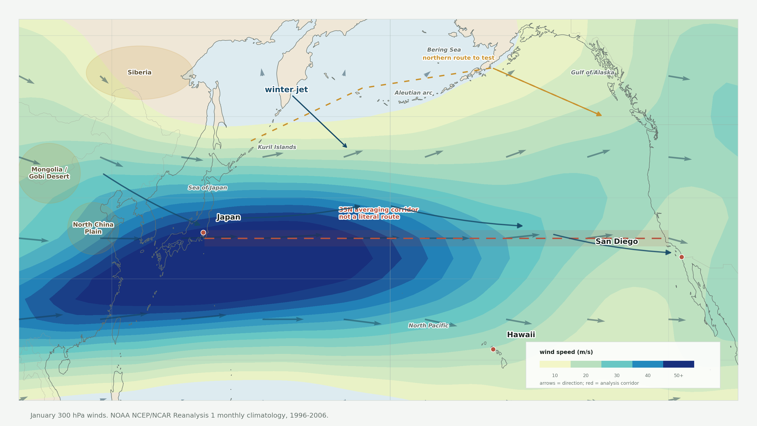
The lead map is the first sanity check. The red line is not meant to be a literal path from Japan to San Diego. It is the 35N averaging corridor used to summarize west-to-east flow. The more interesting geography is the broader winter setup: upstream Asia into Japan, then trans-Pacific westerlies toward Hawaii and southern California, with a possible northern route around the Aleutians and Gulf of Alaska.
Already narrower than “something in the air” — it gives you places, seasons, and failure modes. If I were turning this into an actual source hunt, I would start with a broad stripe across continental Asia and then try to shrink it.
This is the map I wanted: not a claimed source, but a set of specific pins to sample or cross-check against the wind pathway. The terrain and water layers are there to make the sampling question less abstract.
The first pass would be Dunhuang, Dalanzadgad, Lanzhou, Hohhot, Beijing, Shenyang, Changchun, Harbin, Seoul, and Tokyo. I would not treat those as magic dots on a map. I would treat them as places to pull soils, dust, crop residue, fungi and yeasts, toxins, and fine aerosols into the same comparison frame.
I also want the map to show what the air is passing over. Rivers, lakes, basins, deserts, mountains, and nearby cities change the list of plausible things to check. A dust-source basin is not the same sampling problem as a river valley, an agricultural plain, or a downwind city.
The extra city labels are there as anchors, not as accusations: Almaty and Oskemen on the Kazakhstan side; Ulaanbaatar, Sainshand, and Choibalsan in Mongolia; and Irkutsk, Chita, Blagoveshchensk, Khabarovsk, and Vladivostok across the southern Russian edge of the map.
I would treat that stripe as a sampling plan. The desert regions matter because Asian dust-source areas can loft bacterial and fungal bioaerosols (Maki et al., 2019). The North China and northeast China pieces matter because later flight sampling over Japan, designed around suspected source-region winds, found a strong fungal signal including Candida, while still stopping short of naming a causal agent (Rodo et al., 2014). The agricultural and soil regions matter because toxins, plant decay, fungi, yeasts, and dust-attached cofactors are all different enough that I would not want one generic “upstream Asia” bucket.
What the biology says to look for
Before sampling anything in the swath, it helps to ask what Kawasaki disease itself tells you about the agent. The geography exercise above gives you a search area; the immunology gives you a search criterion. You need both before sampling starts to mean anything.
The immune picture gives a few constraints. Affected arterial tissue in KD cases shows oligoclonal IgA plasma cells — the kind of antibody response associated with mucosal surfaces, especially respiratory ones (Rowley et al., 1997). That points toward inhalation as the entry route, not ingestion or contact. The response is also antigen-driven and intense enough to cause systemic vasculitis in otherwise healthy young children, which fits two mechanisms: a conventional response to a highly immunogenic protein, or a superantigen response. Superantigens — a class that includes certain bacterial and fungal proteins — bypass normal T-cell selection and activate a disproportionately large fraction of T cells at once, meaning a small inhaled dose can drive a much larger immune cascade than you would expect (Leung et al., 1993). Children with limited prior exposure are more vulnerable, which would also explain why adults rarely present with full Kawasaki disease: earlier low-level encounters may have already built partial tolerance.
The geography gives you a search area. The immunology gives you the search criteria. A candidate that satisfies the geography but fails any of these four filters is not a viable hypothesis.
Survival through trans-Pacific transport is the second filter. The pathway runs at altitude over five to ten days. Naked respiratory viruses mostly do not survive that. Fungal spores do — thick walls, low metabolic activity, UV tolerance. Bacterial endospores do. Stable proteins or toxins bound to mineral dust particles do. The candidate field narrows: you are more likely looking for a spore, a heat-stable protein, or a toxin riding a dust particle than for a fragile infectious agent. Coxiella burnetii is the most-documented example of a pathogen that survives long-range aerosol transport — its resistance to desiccation and UV is exceptional, and Q fever outbreaks have been traced to wind-dispersed aerosols from livestock operations at distances of tens of kilometers (Tissot-Dupont et al., 2004).
The 2014 Rodo flight-sampling work found elevated Candida concentrations in air samples over Japan during high-P-WIND conditions (Rodo et al., 2014). Candida can behave as a superantigen and produces protein antigens stable enough to survive aerosolization. Not a confirmation — there was a lot in that air — but it puts yeast and dimorphic fungi at the front of the biological candidate list.
Those constraints make the swath stations meaningfully different problems:
- Dunhuang and Dalanzadgad are desert-edge stations. The priority there is dust-source fungi and Coxiella burnetii. The Gobi steppe supports enough livestock to be a plausible reservoir, and Coxiella’s aerosol hardiness makes it worth checking even at distance.
- Lanzhou, Hohhot, and the Yellow River basin combine loess dust with agricultural soil and river-valley humidity — conditions that favor Fusarium and Alternaria, both of which produce stable mycotoxins alongside viable spores.
- Northeast China (Shenyang, Changchun, Harbin) is a major corn, soybean, and wheat belt. Harvest-season disruption is behind you by January, so the sampling priority shifts toward overwintering soil fungi, decaying crop residue, and toxins that persist well after harvest.
- Seoul and Tokyo are validation endpoints rather than source candidates. If upstream stations show elevated fungal aerosol or mycotoxin concentrations during high-P-WIND months, the question becomes whether those concentrations survive to the downstream sites at levels that matter.
One thing I keep returning to: if the superantigen mechanism is correct, the sampling target changes. You are not necessarily looking for live pathogen counts. You are looking for protein concentrations stable enough to reach the respiratory mucosa of a young child at a biologically active dose. That is a different assay than culturing whatever grows from a dust grab sample, and it would be easy to miss the signal entirely if you only ran one type of screen.
A second complication compounds this. The atmosphere over East Asia is not a passive conveyor belt. During five days of winter transit, particles undergo continuous chemistry. Industrial SO₂ from NE China’s coal and steel sector reacts with ammonia volatilized from livestock and agricultural soils to form ammonium sulfate aerosol. Organic compounds from crop residue and soil react with ozone and UV radiation to form secondary organic aerosols that did not exist at the source. Organochlorine residues on mineral dust surfaces photolyze and undergo oxidation reactions. Biological material — spore coatings, protein fragments, cell-wall components — can adsorb onto inorganic particles, change their immunological surface, and arrive at the receptor site as something chemically distinct from anything you would find in a source-region grab sample. This matters for study design: sampling only at the upstream end and then looking for the same compound at the downstream end may consistently miss a reaction product that forms during transit. The Rodo flight-sampling work — which sampled air over Japan rather than at the source — sidesteps this problem by measuring what is actually present at the destination. That is one reason it remains the most directly relevant dataset in the literature, even though it did not identify the agent.
What leaves the source and what arrives at the receptor are chemically different. This is why source-region grab samples can systematically miss the actual exposure, and why flight sampling over Japan — however imperfect — captures something no ground-based sampling of the upstream region can.
Turning wind into a number
To compare wind with disease timing, you need to turn the map into something repeatable. The paper does that with wind indices. Rodo and coauthors define P-WIND as the mean zonal wind along 35N from 140E to 240E; their seasonal case comparison shows it at the surface, with similar behavior reported in the middle and upper troposphere (Rodo et al., 2011).
For this post I used the same corridor idea, but the map and animation use the 300 hPa upper-air field. I ran the indices at 500 hPa first — the mid-troposphere — and the corridor was present but muddier, with the Asian continent sector blurring into the Pacific transition zone. The switch to 300 hPa sharpened it considerably. That sharpening matters: if the signal were just “winter westerlies at any altitude,” it would be less distinctive than something specific to the jet level. The three indices:
- P-WIND here: mean 300 hPa east-west wind along 35N, 140E-240E.
- Japan NW-WIND here: 850 hPa wind projected onto a northwest/southeast axis over 30-45N, 130-145E.
- Period: 1996-2006 monthly climatology from NOAA reanalysis.
This is the compression step. A big moving atmosphere becomes two monthly signals I can actually compare and try to break.
In this reconstruction, P-WIND peaks in February at about 42.94 m/s and bottoms out in August at about 5.55 m/s. Japan NW-WIND peaks in January at about 7.68 m/s and bottoms out in August at about 0.24 m/s. The exact numbers are less important than the shape. The wind is not a flat background. It has a seasonal pulse.
The pathway question
The monthly wind field is where the idea becomes easier to argue with. The moving dots below are not a simulation of the causal agent. They are tracer pulses pushed by the monthly 300 hPa wind field, which makes the open corridor easier to see and keeps the upstream inspection areas on the map.
The gold areas are where I would start looking upstream. The moving dots follow the wind field so the winter pathway reads like motion instead of a static weather map.
I would not call that a mechanism. I would call it a better target. If there is a transported trigger, I would start looking upstream of Japan and then along the winter Pacific corridor toward Hawaii and southern California. I would also keep the northern Pacific branch in play, because the paper itself treats the atmospheric path as more than one clean line across the ocean.
The thing to look for is not just “aerosols” in the abstract. It is a candidate exposure that appears in the right upstream region, survives the relevant atmospheric conditions, and shows up when the pathway is open. A much harder claim, but at least one you can actually test.
Where the guess begins
This is where I would draw the line. The paper shows a recurring alignment between disease timing and wind structure. My rebuild shows that the atmospheric part of that story is real enough to reproduce. None of that identifies the agent.
This is the useful output: a search area, not a proof chain.
The easy move is to either sell this as “wind causes Kawasaki disease” or write it off as seasonal correlation dressed up with a good map. Neither is right. The atmospheric side is specific enough to be a research lead — worth taking seriously as a target, not worth promoting to a mechanism before you have tried to break it.
What testing has ruled out
The atmospheric case is specific enough to take seriously. But before hunting for the agent, it is worth being precise about what systematic testing has already eliminated — and what the eliminations imply about what is left.
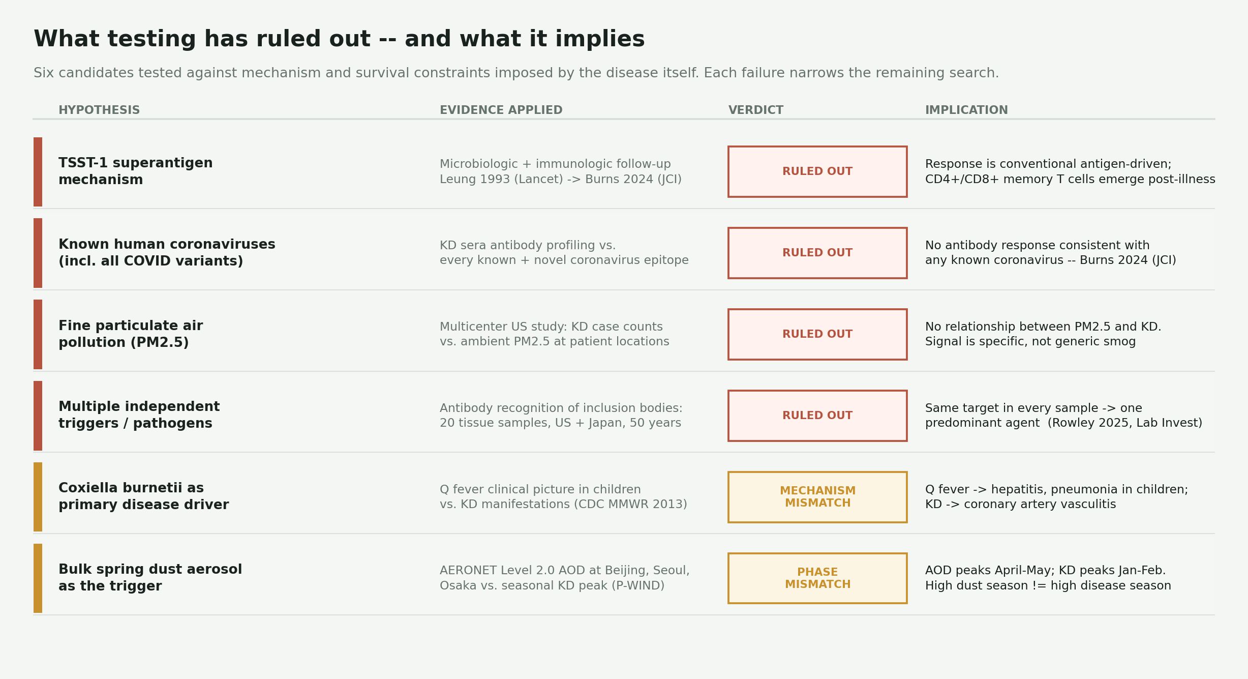
Six candidates, each tested against a specific mechanism or survival constraint. The failures are as informative as the positives: they eliminate entire classes of explanation and push the remaining candidates toward a narrow, testable profile.
TSST-1 and the superantigen hypothesis. In 1993, Leung and colleagues reported that TSST-1-secreting Staphylococcus aureus was found in most KD patients but rarely in controls, proposing a superantigen mechanism (Leung et al., 1993). It was a reasonable hypothesis — superantigens bypass normal T-cell selection and can drive disproportionately large immune cascades from small inhaled doses. The hypothesis attracted follow-up work for a decade. A 2024 review in the Journal of Clinical Investigation concluded that “more detailed microbiologic and immunologic studies failed to support the existence of a superantigen as a driver of the acute inflammatory state in KD,” with evidence now consistent instead with “an appropriate immune response to a conventional antigen with the emergence of both CD4+ and CD8+ memory T cells following the acute illness” (Burns, 2024). The mechanism is ruled out; what it implies is that you are looking for something highly immunogenic but functioning through normal antigen-presentation pathways.
Known human coronaviruses. Every known and novel coronavirus was screened against antibody profiles from KD patient sera. The same 2024 JCI review states that “antibody profiling of KD sera has failed to reveal a response consistent with known or novel human coronaviruses.” A natural experiment reinforced this: during the COVID-19 pandemic, common respiratory viruses in children essentially disappeared from circulation — influenza, RSV, and endemic coronaviruses all dropped sharply — while Kawasaki disease continued without a corresponding change in incidence or age distribution. Whatever causes KD was not affected by the same contact-reduction measures that eliminated the usual respiratory viruses.
Fine particulate air pollution (PM2.5). A multicenter US study found no relationship between ambient PM2.5 concentrations and KD case counts (Burns, 2024). This matters because it separates the story from generic air-quality explanations. The signal is not “wherever there is particulate pollution, there is more Kawasaki disease.” It is specific in geography and season in a way that industrial smog cannot produce.
Multiple independent triggers. The most recent direct pathology evidence changes the framing considerably. Rowley and colleagues prepared monoclonal antibodies from blood cells of KD patients and tested them against twenty tissue samples from deceased patients in the US and Japan spanning fifty years. Every one of the twenty samples showed the same cytoplasmic inclusion bodies — characteristic by-products of viral infection — recognized by the KD antibodies (Rowley et al., 2025). The inclusion bodies were located in medium-size airways, indicating a respiratory entry route. Fifty years of US and Japanese cases, the same target in every autopsy sample: this pattern is not consistent with multiple different pathogens or environmental toxins. It points to one predominant agent.
Coxiella burnetii as the primary mechanism. The aerosol hardiness of C. burnetii, its livestock reservoir in northeastern China and Kazakhstan, and its documented long-range wind dispersal make it a plausible candidate for the transport pathway (Tissot-Dupont et al., 2004). But the clinical picture does not fit the disease. Q fever in children presents primarily as hepatitis and pneumonia; coronary artery vasculitis is not part of its known clinical spectrum in pediatric cases (CDC MMWR, 2013). Large-vessel vasculitis from C. burnetii has been described in rare adult cases, but coronary artery aneurysms in young children — the defining feature of Kawasaki disease — are not. The reservoir geography and aerosol survival are right; the disease mechanism is wrong.
Bulk spring dust aerosol as the transport vehicle. The AERONET data from Beijing, Seoul, and Osaka is direct on this: aerosol optical depth peaks in April and May — the Asian dust season driven by spring thaw, agricultural tillage, and convective lofting — while P-WIND and Kawasaki disease both peak in January and February. A two-to-three month phase offset rules out bulk spring dust load as the driver. Whatever is being transported during the winter jet pulse is not the same material that dominates spring aerosol over East Asia.
What remains. After these eliminations, the remaining candidate profile is narrow: a single, novel respiratory pathogen — almost certainly a virus, given the inclusion body evidence — with sufficient environmental stability to survive five to ten days of winter trans-Pacific transport at altitude. It triggers a conventional antigen-specific immune response rather than a superantigen cascade. It enters through the respiratory mucosa, consistent with the IgA plasma cell infiltration of proximal respiratory tissue documented by Rowley and colleagues in earlier work (Rowley et al., 1997). And its source region, based on the back-trajectory analysis, is northeastern China and Mongolia during the winter jet season.
That is a narrow enough profile to be testable. It is also nothing like the common respiratory viruses that circulate globally in winter — which is why Kawasaki disease has such a different epidemiology from influenza, RSV, and coronavirus.
The emergence problem
One question that rarely comes up in the wind-pathway literature: when did Kawasaki disease actually start?
The epidemiology answer is unsatisfying. A retrospective review of pediatric records at Tokyo University Hospital found no convincing KD cases before 1950 and identified only a handful in the early 1950s — a pattern the authors describe as the disease being rare or nonexistent prior to that decade (Shibuya et al., 2002). Dr. Kawasaki’s first confirmed patient was a four-year-old boy in January 1961. By the time he published his 50-case series in 1967, the disease had become recognizable enough that colleagues knew what he was describing. By 1970, Japan had launched a formal biennial national surveillance program. The three major epidemics — 1979, 1982, 1986, each roughly doubling the case count of the preceding year — suggest a disease that is not static but is responding to something that varies interannually (Burns, 2018).
There is a competing explanation for the 1950 emergence that I cannot rule out from wind data alone. Japanese repatriation from mainland China and Korea was massive in the late 1940s — roughly six million people returned in the years after 1945. If the causative agent is endemic to Northeast China, returning soldiers and civilians could have introduced it to Japan via person-to-person exposure or contaminated goods, entirely separately from the wind pathway. That hypothesis predicts cases should appear regardless of P-WIND values after 1945, while the wind hypothesis predicts incidence should track the atmospheric corridor. The epidemics in 1979, 1982, and 1986 — which are interannual spikes rather than a steady level — favor the wind mechanism for those events, since repatriation was long over by then. But the initial emergence in the 1950s remains ambiguous.
That ambiguity noted, the timing of what was happening upstream is still hard to ignore.
1953–1957. China’s First Five Year Plan, backed by 156 Soviet-assisted industrial projects. Fifty-eight of those projects were concentrated in Northeast China — Shenyang, Harbin, Changchun, Anshan, Fushun. The Anshan steel complex, already the largest in China, expanded massively. Fushun coal output eventually accounted for ten percent of national production. These were not incremental changes. Within a decade, the same region that would later be identified as the probable source zone for the Kawasaki wind pathway went from a patchwork of post-war reconstruction to one of the most heavily industrialized landscapes on earth, with essentially no air-quality controls.
1953–1965. Khrushchev’s Virgin Lands Campaign plowed up more than 40 million hectares of Kazakh steppe — much of it at the western edge of our source swath. Wind erosion was catastrophic from the start. In 1956–1958 alone, more than ten million hectares of topsoil blew away from newly broken fields (Morozova et al., 2021). Livestock herds grew rapidly alongside the settler population. Both factors are relevant here: soil disturbance lofts previously buried fungal communities, and large livestock populations on denuded steppe are a canonical reservoir for Coxiella burnetii. Anthrax outbreaks in Kazakhstan during the campaign are documented (Bakyt et al., 2025); Q fever exposure was almost certainly rising in parallel.
1957–1964. The Great Leap Forward stripped at least a third of China’s forests, with Manchuria among the worst-affected regions. Deep ploughing campaigns, grassland conversion to farmland, and the destruction of windbreaks all compounded the industrial aerosol load with a new and massive dust source. Soils that had been stabilized by forest cover for centuries were suddenly exposed. The specific fungal communities in Manchurian forest soils — Fusarium, Candida relatives, dimorphic species — would have been disturbed and aerosolized on a scale that had no historical precedent.
Three overlapping land-surface disruptions across the source swath, 1950 to 1967. The industrial belt arrives first, then the Virgin Lands Campaign begins lofting Kazakh steppe soil westward of the swath, then the Great Leap Forward strips Manchurian forest cover on its eastern edge. Japan’s first recognized Kawasaki case appears in 1961 — within the decade when the upstream land surface was being transformed faster than at any point in the region’s recorded history.
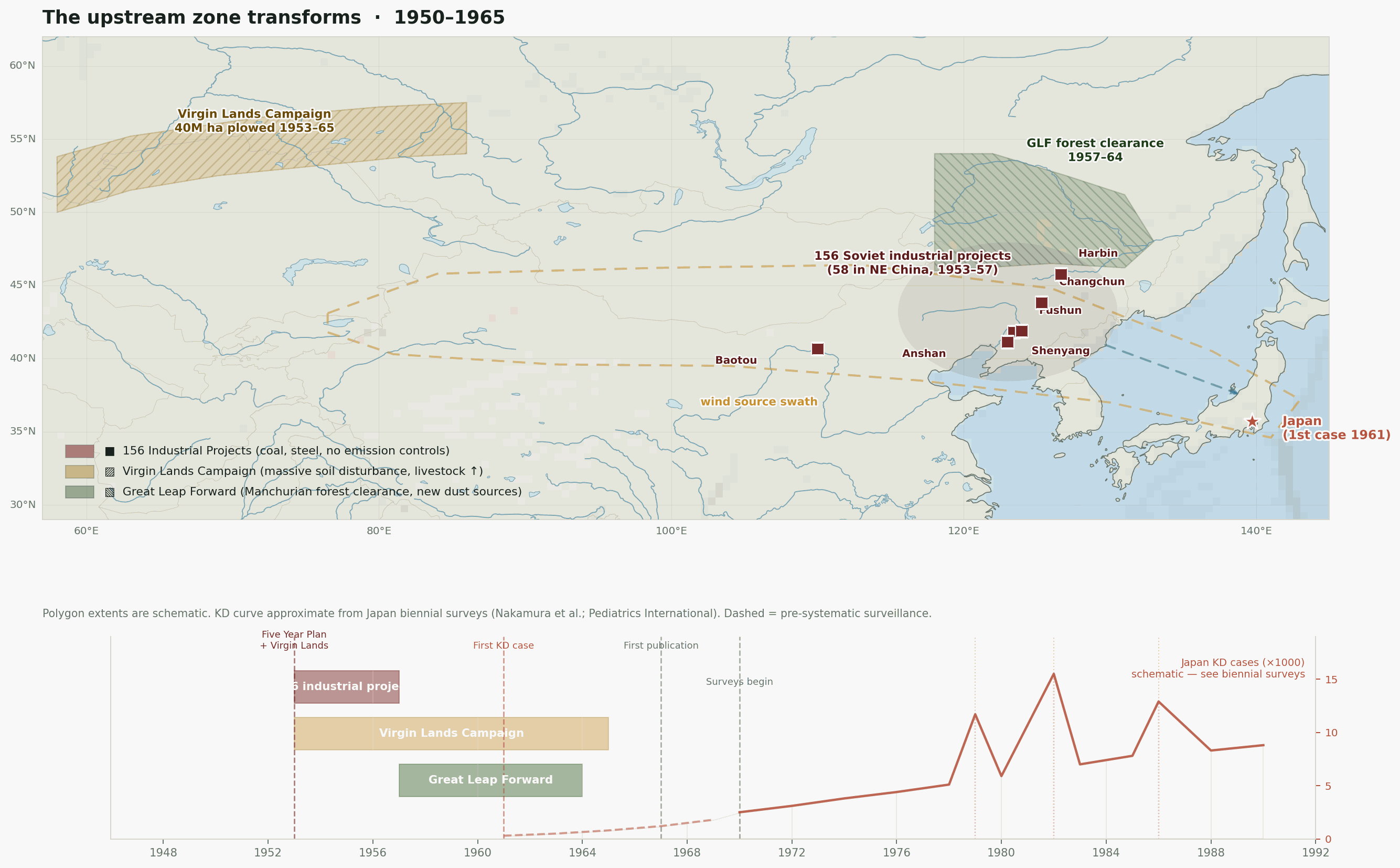
Figure 4. Geographic context for the emergence problem. Three large-scale land-surface disruptions occurred in the source swath within a decade of the disease’s first documented appearance in Japan. The source swath outline corresponds to the corridor identified by Rodo et al. (2011). Epidemic year markers are from Japanese national KD surveillance.
The agricultural chemical layer. This is a thread I have not seen examined in the KD literature. Post-1949 China launched mass pesticide campaigns using organochlorines — DDT and hexachlorocyclohexane (HCH/BHC) — applied at scale across the Northeast agricultural belt from the 1950s through the 1970s. China accounted for roughly 33% of world HCH production and 20% of DDT production between 1950 and 1983, the overwhelming majority of it applied domestically, with Liaoning Province — Shenyang, Anshan, Fushun; the core of our source swath — identified as a major center of both production and agricultural application in retrospective soil surveys (Li et al., 2008).
Before going further: DDT was used globally in the same period. The US, Europe, and much of the developing world were also saturated with organochlorines in the 1950s–70s, and Kawasaki disease does not appear in those places at anything close to the incidence it reaches in Japan. So organochlorines alone cannot be the causal variable. The geographic specificity of KD points to something that is particular to the NE China source zone — not to organochlorine exposure as a universal chemical trigger.
What the chemical layer might contribute is more subtle: selective pressure on soil microbial communities. Organochlorines are toxic to many bacteria and soil invertebrates but less so to certain fungal lineages, including some that produce heat-stable proteins and superantigen-like compounds. Applied at Liaoning-scale concentrations on Manchurian black soil — which has a distinct native fungal community shaped by centuries of cold-deciduous forest ecology, not shared with the US Corn Belt or European wheat fields — the competitive outcome could differ. That is a hypothesis, not a finding. What makes it testable: Chinese organochlorine soil concentration data by province exists in the literature, and the native soil fungal community in Manchurian agricultural land has been characterized. Overlaying those against each other, and against the P-WIND index, is a concrete open-data step, not a request for new sampling.
The synthetic nitrogen fertilizer layer is more quantitatively grounded. China’s nitrogen fertilizer consumption in 1952 was negligible; by 2008, it had grown 25-fold, from roughly 2 to 60 million metric tonnes per year (Yu et al., 2022). The growth was concentrated in the 1970s onward as Green Revolution variety adoption spread through the Northeast corn-soybean belt. High nitrogen loading can shift soil fungal communities toward fast-growing decomposers, including Fusarium and related genera that produce both viable spores and mycotoxins. The FAO fertilizer database and the provincial-level Chinese agricultural statistics (available from 1987 forward) would let you separate the Northeast application trend from the national average — and compare it against the Japan KD incidence curve from the same period. That correlation does not exist in the published literature, as far as I can find.
What the timeline suggests. The disease that did not exist before 1950 began appearing in Japan in the early 1960s, within a decade of the most rapid and large-scale transformation of the upstream land surface in the region’s recorded history. Case counts rise through the 1970s as industrial output and agricultural intensification in Northeast China both continue to grow. The three epidemics in 1979, 1982, and 1986 are preceded, in each case, by anomalous wind patterns that shift the airflow over Japan to a more northwesterly origin during the preceding fall and winter (Rodo et al., 2011).
None of this is a proof. The disease could have existed before 1950 and simply not been diagnosed. The correlation could be coincidental — a lot of things changed after 1950. But the specificity of the geography, the timing of the emergence, and the character of the land-surface change in the source zone all point in the same direction. It is the kind of convergence that warrants at least checking against the historical record before dismissing it.
One thing that could be done without any fieldwork: pull China’s industrial output index and Northeast China agricultural area data by decade, overlay them against the Japan KD incidence curve from the biennial surveys (available from 1970), and test whether the long-term trend is better explained by the P-WIND index alone or by P-WIND combined with an upstream land-use intensity proxy. If the combined model fits and the land-use proxy adds signal independent of the wind index, that is a more specific claim than anything currently in the literature.
What I would do next
I would try to break the pathway before I tried to defend it.
First, run back-trajectory analysis from Japan, Hawaii, and San Diego during peak Kawasaki months and see whether the upstream air actually originates from the swath region. This is the step most likely to kill the idea quickly, which is exactly why I would do it first.
Second, stress-test the index. Recompute P-WIND across nearby pressure levels and corridor windows. I am less confident about the northern route around the Aleutians — I would want to know whether it produces a different seasonal timing or the same one as the main corridor before treating them as one thing.
Third, negative controls. If the same P-WIND index lights up every winter respiratory illness, the idea is weak. If it stays specific to Kawasaki disease timing at the geographic locations the paper identifies, that is a different situation. I do not know which it is, and I would not skip that test.
Fourth — and this is where I would need people with actual field capacity — compare the index with aerosol and environmental sampling from upstream stations during high-P-WIND months, using assays that can detect protein antigens and mycotoxins and not just cultivable organisms. The 2014 Rodo flight-sampling work is the closest existing data point, and even that stopped short of a confirmed agent.
A workflow from the public record
You do not need soil samples or flight-sampling capacity to start narrowing this. Several of the key questions are answerable from publicly accessible satellite data, atmospheric modeling tools, and published case records. Here is how I would structure that analysis, in order of what is most likely to kill the hypothesis quickly.
Steps 1 and 5 are the decision points. If back-trajectories scatter randomly during epidemic years, the spatial story is wrong — no further work is needed. If P-WIND predicts influenza timing as well as Kawasaki disease timing, the index is a winter proxy, not a specific transport signal.
Step 1 — Back trajectories from the downstream sites
NOAA’s HYSPLIT model (available through the READY web interface without an account) lets you run back-trajectory ensembles from any point on earth for any date in the reanalysis record. The starting points are Yokohama or Osaka for Japan, Honolulu for Hawaii, and San Diego for California. The starting dates are January through March for both epidemic and non-epidemic years in the Japan Kawasaki dataset.
Japan’s national Kawasaki disease surveys have been published by the Japan Kawasaki Disease Research Committee since 1970 and appear periodically in Pediatrics International. The epidemic years — 1979, 1982, and 1986 — are well-established and give you specific high-case periods to test against non-epidemic years with similar wind climatology. The test: do trajectories from the downstream sites during high-case months cluster over the Northeast China and Gobi region more than trajectories from low-case years? If they scatter regardless of Kawasaki timing, the spatial story is in trouble. If they consistently trace back to the upstream swath during epidemic peaks, it holds.
Step 2 — Aerosol load in the upstream region
NASA’s MODIS instruments on Terra and Aqua have measured aerosol optical depth (AOD) globally since 2000. NASA’s Giovanni portal lets you pull seasonal AOD maps for any geographic bounding box and time period in a browser without downloading anything. The question is whether AOD over the Northeast China and Gobi sectors is elevated during high-P-WIND months relative to low-P-WIND months, and whether interannual AOD variation in the upstream region tracks the downstream Kawasaki case signal at all.
CALIPSO goes further: it provides vertical aerosol profiles and can classify aerosol type — dust versus smoke versus other. If the upstream signal is dominated by mineral dust during the relevant months, that narrows the hitchhiking candidates toward dust-bound material rather than free-floating spores.
MERRA-2, NASA’s atmospheric reanalysis, has explicit dust emission and transport fields going back to 1980. You can pull dust column mass density over the swath for any year and check whether dust emission in the source zones peaks contemporaneously with the P-WIND index and the Kawasaki case timing. The Gobi and Taklimakan dust emission fields from MERRA-2 are granular enough to distinguish the Gobi desert edge from the loess plateau from the agricultural northeast, which maps directly onto the site-priority breakdown above.
Step 3 — Characterize the upstream land without visiting it
Without sampling, you can still characterize what the wind is passing over. The FAO Global Livestock Density maps give pastoral grazing intensity across the Gobi and Inner Mongolia steppe. High grazing density in the upwind zone raises the prior for Coxiella burnetii as a candidate — it needs a livestock reservoir and is documented for long-range aerosol transport — enough to justify checking Coxiella-specific assay results against the wind index if such data exist in the literature.
For the Northeast China agricultural belt, ESA CCI Land Cover and FAO GeoNetwork both provide dominant crop types at district resolution. The corn and soybean belt running from Shenyang through Harbin is a high Fusarium pressure zone. Cross-referencing crop type with the January P-WIND index at least tells you whether the air during the transport window is coming from over fields that were producing mycotoxin-generating fungi the previous growing season.
NASA FIRMS tracks active fires and burn area globally from 2000 onward. Northeast China agricultural burning — post-harvest residue burning — peaks in October through November. If burn aerosols were a primary mechanism you would expect a different seasonal lag than the January-February Kawasaki peak. FIRMS makes that check trivial.
Step 4 — Pollution and industrial emission overlays
The Global Burden of Disease air pollution layers and the WHO Ambient Air Quality Database both have PM2.5 and PM10 concentration estimates at national and subnational resolution. These are less useful as causal candidates than as confounders to rule out: if Kawasaki case timing correlates with industrial PM2.5 from Chinese manufacturing corridors rather than with dust from the Gobi edge, that is a different hypothesis. Layering industrial emission source maps from the EDGAR database against the swath would help distinguish dust-source zones from combustion-source zones.
Sentinel-5P TROPOMI (available through the Copernicus browser) provides tropospheric columns for NO₂, SO₂, formaldehyde, and aerosol index at 3.5 km resolution. Monthly composites show the extent to which the Northeast China agricultural belt and the Yellow River industrial corridor are contributing aerosol versus the cleaner desert-edge upwind regions. If the transport pathway runs through a heavily industrialized column, you want to know whether that contaminates the biological signal.
Step 5 — Negative controls
This is the step that decides whether the signal is meaningful. Pull the P-WIND index for the same months and the same Japan locations and compare it against seasonal timing for influenza, respiratory syncytial virus, and rotavirus — illnesses with strong winter seasonality in Japan that should have no trans-Pacific wind mechanism. Seasonal case data for influenza and RSV in Japan are published by the National Institute of Infectious Diseases.
If P-WIND predicts all of them equally well, it is probably a proxy for “winter in Japan” rather than a specific transport signal. If it tracks Kawasaki timing better than those diseases — particularly in interannual variation — the specificity is real. The same logic applies geographically: Kawasaki incidence in landlocked regions that sit upwind of the swath rather than downwind should not track with P-WIND. Those are natural negative controls on the geography.
What a positive result looks like at this stage
Not a proof, and not a mechanism. A positive result here is: back trajectories cluster upstream during epidemic years, MODIS and MERRA-2 show elevated dust or aerosol load from high-priority source zones during those periods, the P-WIND index does not equally predict negative-control diseases, and the geographic negative controls do not show the same downstream signal. That combination would justify targeted aerosol sampling along the corridor during a high-P-WIND season — or at minimum a systematic screen of published dust composition literature from stations in the swath during the relevant months.
The open-data workflow does not identify the agent. It narrows the search from the entire upstream stripe to specific zones and specific material types, and it gives you a principled way to decide whether the harder work is worth doing.
What the open-data pass shows
Running the workflow above against publicly available data produces results worth describing honestly — including the things that did not work.
What broke first: the trajectory level. The first version of the back-trajectory code ran at 300 hPa, the same level used for the P-WIND index and the animation. Seven-day trajectories at 300 hPa speeds (30–50 m/s in winter) move 18,000 to 30,000 km backward in time — roughly 160 to 270 degrees of longitude. Starting from Japan, that puts January origins somewhere over Kazakhstan or the Middle East, which is physically absurd for any aerosol capable of being deposited in a child’s airways. The jet at that altitude is not transporting surface-emitted material; it is moving above it. The fix was to drop to 850 hPa, the standard low-tropospheric transport level, where winter speeds over East Asia run 5–15 m/s, and shorten the integration to five days. The origins then landed in northeastern China and Mongolia — which is where the Rodo group’s flight sampling put the source region. The 300 hPa version is still in the commit history if you want to see how far wrong a plausible-looking number can take you.
What broke second: the Dunhuang AERONET station. Dunhuang sits at the edge of the Taklimakan desert and is one of the more obvious places to look for dust-source aerosol chemistry. The AERONET Level 2.0 quality-assured data for Dunhuang, downloaded over the 2001–2020 window, returned 21 usable daily observations across the entire nineteen-year period. That is not enough to build a monthly climatology. The station has periods of operation but almost no data passing the Level 2.0 quality thresholds during the winters we care about. This is itself a finding: the site most directly on the Taklimakan edge is the one with the worst data coverage, which means the aerosol composition at that specific location during high-P-WIND months is essentially uncharacterized in the public record. Dunhuang stays on the source-screening map as a sampling priority; it just cannot contribute to the AERONET comparison.
What the API required fixing. The initial AERONET query used Seoul_YONSEI as the station name, which does not exist in the database. Getting the correct name required downloading AERONET’s full station location file and searching for Korean stations — the operating station is Seoul_SNU, attached to Seoul National University. This is not a scientific finding, but it illustrates a real friction point in working with AERONET programmatically: station names are not intuitive, the API returns an empty response rather than an error when the name is wrong, and you can spend time debugging what looks like a data gap before realizing the station name itself is the problem. The script now validates against the location list.
With those corrections in place, the workflow produces two outputs worth discussing.
Back-trajectories confirm the seasonal geography. Five-day 850 hPa back-trajectories computed from NCEP reanalysis winds show that winter air masses over Japan consistently originate from northeastern China and Mongolia — exactly the source swath. January and February trajectories land inside the swath polygon. Summer trajectories are shorter, curve from the south and southeast, and carry no continental Asian land signal at all. The winter pathway is not subtle, and it does not require going all the way to Central Asia to make the argument; the origin is already in the right zone at the aerosol-transport level.
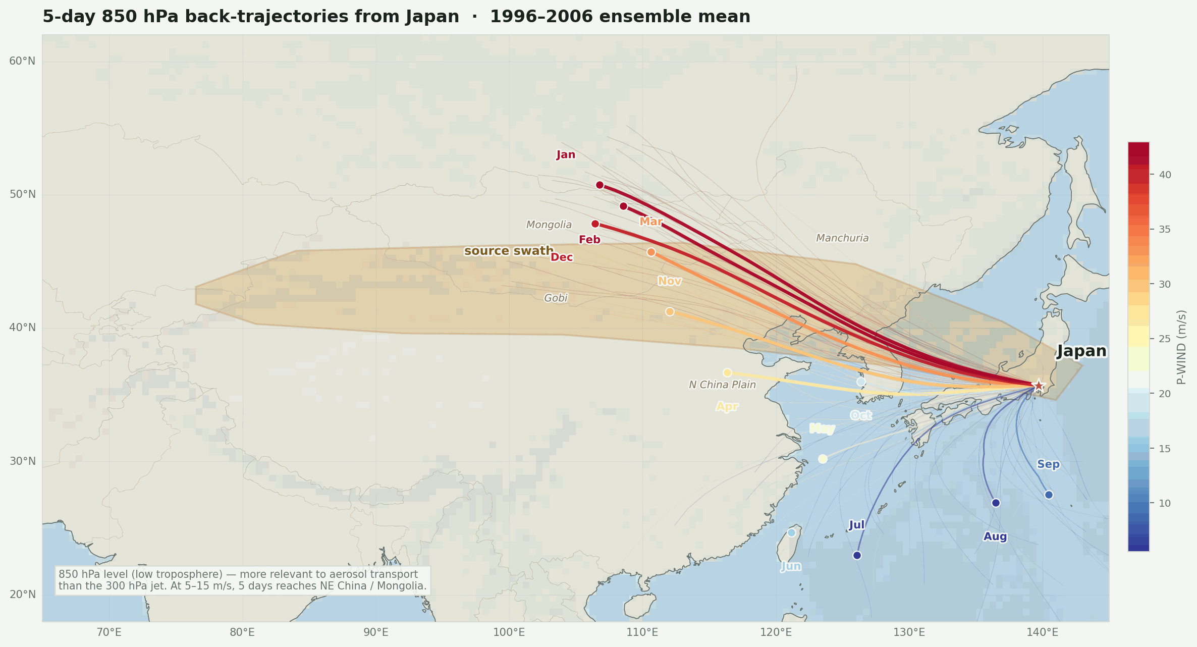
Warm colors (red/orange) are high-P-WIND months — January, February, March. The origin dots land in northeastern China and the Mongolia/Gobi corridor, the same zone flagged by the Rodo group’s flight sampling. Running at 850 hPa keeps the physics honest: this is the aerosol-transport level, not the jet core.
AOD peaks in spring, not winter — and that is interesting. AERONET Level 2.0 daily AOD at Beijing, Seoul, and Osaka all show the same pattern: aerosol optical depth peaks in April and May, not in January or February when P-WIND is highest.
The spring AOD peak is the Asian dust season — thawing soil, agricultural disturbance, increased convective lofting. The winter P-WIND peak is the jet stream at its strongest. These do not coincide.
That mismatch matters. If the Kawasaki signal were driven by dust aerosol concentration at the source, you would expect the downstream disease peak to align with spring AOD, not winter P-WIND. The fact that it aligns with P-WIND and not AOD points away from bulk dust load as the mechanism and toward something that is specifically transported during the high-velocity winter jet — possibly spores, stable protein complexes, or toxins that do not require a high-dust-emission event to become airborne, or that originate from different source zones than the spring dust basins.
This does not resolve the question. But it does narrow it. If you were designing the aerosol sampling protocol at Dunhuang in January, you would not be looking for the same signal as the spring dust researchers. You would be looking for what is actually in the air when the P-WIND is high and the dust AOD is low — which is a different collection and assay strategy.
Reproducibility note
The wind analysis figures were generated from NOAA PSL NCEP/NCAR Reanalysis 1 monthly wind fields for 1996–2006 using scripts/generate_kawasaki_wind_article_images.py. The back-trajectory and AERONET figures were generated by scripts/kawasaki_open_data_analysis.py, which fetches an 850 hPa wind domain extending west to 65°E for the trajectory integration and downloads AERONET Level 2.0 daily AOD via the public API. Both scripts access NOAA data through OPeNDAP and cache regional subsets under .cache/kawasaki-wind/. Package versions are in requirements-kawasaki-wind.txt.